Code
p_to_z <- function(p) {

  if (p == 1) {
   z = 0
  } else if (p %% 2 == 0) {
   z = p / 2
  } else {
   z = -((p - 1) / 2)
  }

 return(z)

}

# Test with p = 9
p_to_z(p = 9)
[1] -4We say that sets \(A\) and \(B\) are equinumerous if and only if there is a one-one correspondence between \(A\) and \(B\), \(F: A \xrightarrow[onto]{1-1} B\). We shall write \(A \approx B\) to mean that \(A\) and \(B\) are equinumerous.
Theorem D.1 If \(\mathscr{F}\) is an arbitrary collection of sets where \(A \in \mathscr{F}\), \(B \in \mathscr{F}\) and \(C \in \mathscr{F}\) then \(\approx\) is an equivalence relation on \(\mathscr{F}\):
Proof.
Let \(I_A: A \longrightarrow A\) be the identity function on \(A\) where \(I_A(x) = x\) for all \(x \in A\). Because \(I_A: A \xrightarrow[onto]{1-1} A\) then \(A \approx A\).
If \(A \approx B\) then there is a \(F\) such that \(F: A \xrightarrow[onto]{1-1} B\). By Theorem 1.11 \(F^{-1}: B \xrightarrow[onto]{1-1} A\) so \(B \approx A\).
If \(A \approx B\) and \(B \approx C\) there exist \(F\) and \(G\) such that \(F: A \xrightarrow[onto]{1-1} B\) and \(G: B \xrightarrow[onto]{1-1} C\). By Corollary 1.4 \(G \circ F: A \xrightarrow[onto]{1-1} C\), so \(A \approx C\).
Exercise D.1
If \(A \approx \emptyset\) prove that \(A = \emptyset\)
Prove that \(A \approx A \times {y}\) (Hint: Let \(\theta(a) = (a,y)\) for all \(a \in A\))
Solution D.1.
If \(A \approx \emptyset\) then \(F: A \xrightarrow[onto]{1-1} \emptyset\). Because \(\mathscr{D}(F) = A\) we have that \(\mathscr{D}(F) = \{ x \mid \exists y (F(x) = y)\}\) where \(y \in \mathscr{R}(F)\). However \(\mathscr{R}(F) \subseteq \emptyset\) so \(\mathscr{R}(F) = \emptyset\). Therefore there is no \(y\) such that \(F(x) = y\), which means that \(A\) has no elements. So, \(A = \emptyset\).
Let \(\theta(a) = (a,y)\) for all \(a \in A\). First assume that \(\theta(a) = \theta(b)\) then \((a, y) = (b, y)\). By Exercise 1.32 1 \(a = b\) so \(\theta(a)\) is one-one. Now let any \((a,y) \in A \times \{ y \}\) then \(a \in A\) and \(\theta(a) = (a,y)\) so \(\theta(a)\) is onto. Therefore \(\theta(a): A \xrightarrow[onto]{1-1} A \times \{ y \}\), so \(A \approx A \times \{ y \}\).
Two sets which are equinumerous are said to have the same cardinal number. We assume that each set \(A\) has an associate cardinal number \(\mathscr{K}(A)\). Hence, \(\mathscr{K}(A) = \mathscr{K}(B) \iff A \approx B\).
Definition D.1 If \(\mathscr{F}\) is an arbitrary collection of sets where \(A \in \mathscr{F}\) and \(B \in \mathscr{F}\) the relations \(\leq\) and \(<\) on \(\mathscr{F}\) are defined as:
\(A \leq B \iff \exists F (F: A \xrightarrow[]{1-1} B)\)
\(A < B \iff A \leq B \land A \not \approx B\)
Note: \(A \not \approx B\) means \(\neg(A \approx B)\). Therefore \(A \leq B \land A \not \approx B\) means that \(\exists F (F: A \xrightarrow[]{1-1} B \land \neg(F: A \xrightarrow[onto]{} B))\)
Theorem D.2 If \(\mathscr{F}\) is an arbitrary collection of sets where \(A \in \mathscr{F}\), \(B \in \mathscr{F}\) and \(C \in \mathscr{F}\) then:
\(A \leq A\)
\(A \leq B \land B \leq C \Longrightarrow A \leq C\)
\(A \not < A\)
\(B \subseteq A \Longrightarrow B \leq A\)
\(A \leq B \iff (A < B \lor A \approx B)\)
\(B \leq A \iff \exists W (W \subseteq A \land B \approx W)\)
\((A \leq B \land B \approx C) \Longrightarrow A \leq C\)
\((A \approx B \land B \leq C) \Longrightarrow A \leq C\)
Proof.
Because \(A \approx A\) then there is some \(F: A \xrightarrow[onto]{1-1} A\). Therefore \(F\) is one-one which means that \(A \leq A\).
If \(A \leq B\) and \(B \leq C\) then there exist \(F\) and \(G\) such that \(F: A \xrightarrow[]{1-1} B\) and \(G: B \xrightarrow[]{1-1} C\). By Theorem 1.14 \(G \circ F: A \xrightarrow[]{1-1} C\) so \(A \leq C\).
\(A \not < A\) means that \(\neg (A < A)\). By Definition D.1 b it means that \(\neg (A \leq A) \lor \neg(A \not \approx A)\). Therefore we have that \(\neg (A \leq A) \lor (A \approx A)\). We know by Theorem D.2 that \(\neg (A \leq A)\) is false and by Theorem D.1 that \(A \approx A\) is true. Therefore \(\neg (A \leq A) \lor (A \approx A)\) is true, which means that \(A \not < A\) is true.
By Theorem D.1 \(I_A: A \xrightarrow[onto]{1-1} A\). Therefore \({I_A \mid}_{B}: B \xrightarrow[]{1-1} A\) where \({I_A \mid}_{B}\) is the restriction of \(I_A\) to the domain \(B\) (See Stoll 1974, 40). So \(B \leq A\).
\(\begin{aligned} A \leq B & \iff \exists F (F: A \xrightarrow[]{1-1} B) \\ & \iff \exists F (F: A \xrightarrow[]{1-1} B) \land (\exists F (F: A \xrightarrow[onto]{} B) \lor \neg \exists F (F: A \xrightarrow[onto]{} B)) \\ & \iff (\exists F (F: A \xrightarrow[]{1-1} B) \land \exists F (F: A \xrightarrow[onto]{} B)) \lor (\exists F (F: A \xrightarrow[]{1-1} B) \land \neg \exists F (F: A \xrightarrow[onto]{} B)) \\ & \iff A \approx B \lor A < B \end{aligned}\)
\(\begin{aligned} B \leq A & \iff \exists F (F: B \xrightarrow[]{1-1} A) \\ & \iff \exists F (F: B \xrightarrow[]{1-1} A \land W = \mathscr{R}(F) \subseteq A) \\ & \iff \exists F (F: B \xrightarrow[onto]{1-1} W \land W \subseteq A) \\ & \iff \exists W (B \approx W \land W \subseteq A) \end{aligned}\).
If \(A \leq B\) and \(B \approx C\) there exist \(F\) and \(G\) such that \(F: A \xrightarrow[]{1-1} B\) and \(G: B \xrightarrow[onto]{1-1} C\). By Theorem 1.14 \(G \circ F: A \xrightarrow[]{1-1} C\), so \(A \leq C\).
If \(A \approx B\) and \(B \leq C\) there exist \(F\) and \(G\) such that \(F: A \xrightarrow[onto]{1-1} B\) and \(G: B \xrightarrow[]{1-1} C\). By Theorem 1.14 \(G \circ F: A \xrightarrow[]{1-1} C\), so \(A \leq C\).
We can define an order relation \(<_K\) on cardinal numbers. Let \(\mathfrak{m}\) and \(\mathfrak{n}\) be cardinal numbers. Take any sets \(A\) and \(B\) having cardinal numbers \(\mathfrak{m}\) and \(\mathfrak{n}\) respectively. By Theorem D.2 g and h it does not make any difference in these definitions which sets \(A\) and \(B\) we choose having cardinal numbers \(\mathfrak{m}\) and \(\mathfrak{n}\), respectively.
One can obtain theorems about cardinal numbers analogous to those proved above. For example, the analogue of Theorem D.2 b is \((\mathfrak{m} <_K \mathfrak{n} \land \mathfrak{n} <_K \mathfrak{p}) \Longrightarrow \mathfrak{m} <_K \mathfrak{p}\), for any cardinal numbers \(\mathfrak{m}\), \(\mathfrak{n}\) and \(\mathfrak{p}\).
Theorem D.3 (Cantor theorem) If \(A\) is a set then:
\[A < \mathscr{P}(A)\]
Proof. If \(A < \mathscr{P}(A)\) by Definition D.1 b we need to prove that \(A \leq \mathscr{P}(A) \land A \not \approx \mathscr{P}(A)\).
First, define \(F\) such that \(F(a) = \{ a \}\) for all \(a \in A\) then \(F: A \xrightarrow[]{1-1} \mathscr{P}(A)\) because if \(F(a) = F(b)\) then \(\{ a \} = \{ b \}\) so \(a = b\). Therefore, \(A \leq \mathscr{P}(A)\).
Second, using Note 1.3 assume \(A \approx \mathscr{P}(A)\) so there is some \(G\) such that \(G: A \xrightarrow[onto]{1-1} \mathscr{P}(A)\). Let \(B = \{ b \in A \mid b \not \in G(b) \}\). Because \(B \subseteq A\) then \(B \in \mathscr{P}(A)\) therefore because \(G\) is onto it exists some \(a \in A\) such that \(G(a) = B\). There are 2 possibilities \(a \in B\) or \(a \not \in B\):
If \(a \in B\) then \(a \not \in G(a)\). But \(G(a) = B\) so we have also that \(a \in G(a)\).
If \(a \not \in B\) then because \(G(a) = B\) we have that \(a \not \in G(a)\). However this means that \(a \in B\).
In any case there is a contradiction so it is not the case that \(A \approx \mathscr{P}(A)\). Therefore it must be the case that \(A \not \approx \mathscr{P}(A)\).
Because \(A \leq \mathscr{P}(A)\) and \(A \not \approx \mathscr{P}(A)\) we have that \(A < \mathscr{P}(A)\).
Theorem D.4 (Schröder-Bernstein theorem) If \(A\) and \(B\) are sets then:
\[(A \leq B \land B \leq A) \Longrightarrow A \approx B\]
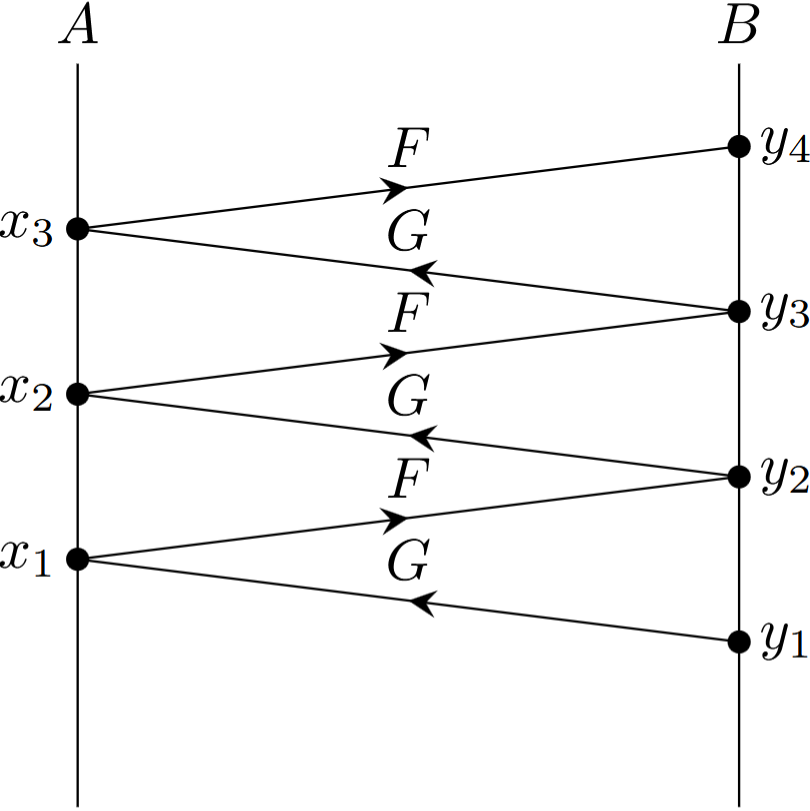
Proof (Based on (Mendelson 2015, 295–96)). Assume \(A \cap B = \emptyset\). If it is not the case we can define \(A_1 = A \times \{ 0 \}\) and \(B_1 = B \times \{ 1 \}\) where by Exercise D.1 2 \(A \approx A_1\) and \(B \approx B_1\) and we can use Theorem D.2 g, h to still prove Theorem D.4.
Let us assume \(F: A \xrightarrow[]{1-1} B\) and \(G: B \xrightarrow[]{1-1} A\). By a B-thread (See Figure D.1) we mean a function \(f\) from the set \(\mathbb{P}\) of positive integers into \(A \cup B\), \(f: \mathbb{P} \longrightarrow A \cup B\), such that:
Therefore \(f(1) = y_1 \in B - \mathscr{R}(F)\), \(f(2) = G(f(1)) \in A\), \(f(3) = F(f(2)) \in B\), \(f(4) = F(f(3)) \in A, \ldots\), \(f(2n) = G(f(2n - 1)) \in A\), \(f(2n+1) = F(f(2n)) \in B, \ldots\).
Thus, a B-thread is an infinite sequence of points starting with a point \(y_1\), which is not in the range of \(F\), and then using the functions \(G\) and \(F\) alternately.
Let \(W = \{ w \in A \mid w \in \mathscr{R}(f) \}\). Then the desired one-one correspondence \(H\) between \(A\) and \(B\) is given by:
\[H(x) = \begin{cases} {G^{-1} \mid}_{W}(x) & \text{if } x \in W \\ {F \mid}_{A - W}(x) & \text{if } x \in W - A \end{cases}\]
Where \({G^{-1} \mid}_{W}\) is the restriction of \(G^{-1}\), that is \(G^{-1}: \mathscr{R}(G) \xrightarrow[onto]{1-1} B\), to the domain \(W\) and \({F \mid}_{W - A}\) is the restriction of \(F\) to the domain \(A - W\) (See Stoll 1974, 40).
We have that:
\[\begin{split} \mathscr{D}(H) & = \{ x \mid \exists y (H(x) = y) \} \\ & = \{ x \mid \exists y ({G^{-1} \mid}_{W}(x) = y \lor {F \mid}_{A - W}(x) = y) \} \\ & = \{ x \mid \exists y ({G^{-1} \mid}_{W}(x) = y) \lor \exists y ({F \mid}_{A - W}(x) = y) \} \\ & = \{ x \mid \exists y ({G^{-1} \mid}_{W}(x) = y) \} \cup \{ x \mid \exists y (F(x) = y) \} \\ & = \mathscr{D}({G^{-1} \mid}_{W}) \cup \mathscr{D}({F \mid}_{A - W}) \\ & = W \cup W - A \\ & = A \end{split}\]
Also because \({G^{-1} \mid}_{W}: W \xrightarrow[]{1-1} B\) where \(\mathscr{R}({G^{-1} \mid}_{W}) \subseteq B\) and \({F \mid}_{A - W}: A - W \xrightarrow[]{1-1} B\) where \(\mathscr{R}({F \mid}_{A - w}) \subseteq B\), we have also that:
\[\begin{split} \mathscr{R}(H) & = \{ y \mid \exists x (H(x) = y) \} \\ & = \{ y \mid \exists x ({G^{-1} \mid}_{W}(x) = y \lor {F \mid}_{A - W}(x) = y) \} \\ & = \{ y \mid \exists x ({G^{-1} \mid}_{W}(x) = y) \lor \exists x ({F \mid}_{A - W}(x) = y) \} \\ & = \{ y \mid \exists x ({G^{-1} \mid}_{W}(x) = y) \} \cup \{ y \mid \exists x (F(x) = y) \} \\ & = \mathscr{R}({G^{-1} \mid}_{W}) \cup \mathscr{R}({F \mid}_{A - W}) \\ & \Longrightarrow \mathscr{R}(H) \subseteq B \end{split}\]
Furthermore, if \(xHy\) and \(xHz\) then \(x{G^{-1} \mid}_{W}y\) and \(x{G^{-1} \mid}_{W}z\) or \(x{F \mid}_{A - W}y\) and \(x{F \mid}_{A - W}z\) but not both. Because \({G^{-1} \mid}_{W}\) and \({F \mid}_{A - W}\) are functions we have that \(y = z\). So \(H\) is also a function. Therefore \(H: A \longrightarrow B\) where now we need to prove that is a one-one correspondence.
First we prove that \(H\) is onto. Let \(b \in B\) then \(G(b) \in W\) or \(G(b) \in A - W\).
If \(G(b) \in W\) then \(H(G(b)) = {G^{-1} \mid}_{W}(G(b)) = b\) taking into account that \(G: B \xrightarrow[]{1-1} A\), \(G^{-1}: \mathscr{R}(G) \xrightarrow[onto]{1-1} B\), \({G^{-1} \mid}_{W}: W \xrightarrow[]{1-1} B\) and \(W \subseteq \mathscr{R}(G) \subseteq A\).
If \(G(b) \in A - W\) then \(G(b) \in A\) and \(G(b) \not \in W\). Also \(H(G(b)) = F(G(b))\) and it must be the case that \(F(G(b)) = b\). Why? If this is not the case then \(b \in B - \mathscr{R}(F)\) so there will be a B-thread such that \(f(1) = b\) where \(G(b) = f(2) \in A\). Therefore \(G(b) = f(2) \in W\) but we have assume that \(G(b) \not \in W\).
Second we prove that \(H\) is one-one. Using Note 1.3 assume that \(H(x) = H(y)\) and \(x \neq y\)
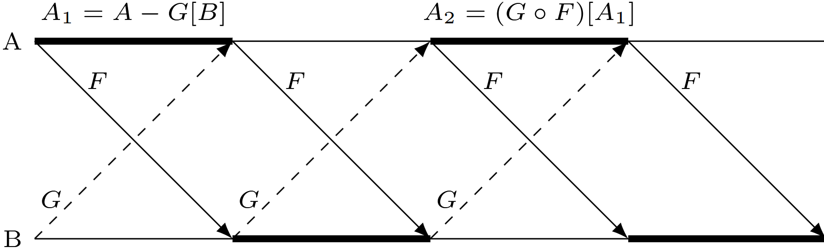
Proof (Based on (Peloquin 2016) and (Enderton 2009, 147–48)). Let \(G: B \longrightarrow A\) and \(C \subseteq B\) then \(G[C] = \mathscr{R}({G \mid}_{C}) = \{ G(c) \mid c \in C \}\) where \({G \mid}_{C}\) is the restriction of \(G\) to the domain \(C\) (See Stoll 1974, 40).
Let \(F: A \xrightarrow[]{1-1} B\) and \(G: B \xrightarrow[]{1-1} A\). Also define \(A_1 = A - G[B]\), \(A_{n+1} = (G \circ F)[A_n]\) and \(A_{\infty} = \bigcup_{n = 1}^{\infty} A_n\) (See Figure D.2).
Now define \(H: A \longrightarrow B\) to be:
\[H(x) = \begin{cases} F(x) & \text{if } x \in A_{\infty} \\ G^{-1}(x) & \text{if } x \in A - A_{\infty} \end{cases}\]
Now we need to prove that \(H\) is a one-one correspondence.
Lets prove that \(H\) is one-one, that is if \(H(x) = H(y)\) then \(x = y\)
If \(x\) and \(y\) are in \(A_{\infty}\) because \(F\) is one-one then \(H(x) = F(x)\) and \(H(y) = F(y)\) so \(F(x) = F(y)\) implies that \(x = y\)
If \(x\) and \(y\) are in \(A - A_{\infty}\) by Theorem 1.11 \(G^{-1}: \mathscr{R}(G) \xrightarrow[onto]{1-1} B\). So \(G^{-1}\) is one-one, which means that \(H(x) = G^{-1}(x)\) and \(H(y) = G^{-1}(y)\) so \(G^{-1}(x) = G^{-1}(y)\) implies that \(x = y\).
If \(x \in A_{\infty}\), \(y \in A - A_{\infty}\) and \(H(x) = H(y)\) then \(F(x) = G^{-1}(y)\). Therefore \(G(F(x)) = G(G^{-1}(y)) = y\), so \(G(F(x)) = y\). Because \(x \in A_{\infty}\) then \(x\) belongs to some \(A_n\) so \(G(F(x)) \in A_{n + 1}\). Therefore \(y \in A_{n + 1}\) and \(y \in A_{\infty}\). However this is a contradiction because we assume that \(y \in A - A_{\infty}\). This means that we need to discard this case.
Therefore \(H\) is one-one.
Lets prove that \(H\) is onto, that is for any \(b \in B\) it exists \(a \in A\) such that \(H(a) = b\). Because \(G: B \xrightarrow[]{1-1} A\) then \(G(b) \in A - A_{\infty}\) or \(G(b) \in A_{\infty}\).
If \(G(b) \in A_{\infty}\) then \(H(G(b)) = G^{-1}(G(b)) = b\). So \(H(G(b)) = b\) where \(G(b) \in A\)
If \(G(b) \in A_{\infty}\) then \(G(b)\) belongs to some \(A_n\). It can not be \(A_1 = A - G[B]\) because \(G(b) \in G[B]\). So \(G(b)\) must belong to some \(A_{n+1} = (G \circ F)[A_n]\). Therefore we have that \(G(b) = G(F(a))\) for some \(a \in A_n\), so \(a \in A_{\infty}\). Then we have that \(b = G^{-1}(G(b)) = G^{-1}(G(F(a))) = F(a) = H(a)\) because \(a \in A_{\infty}\). So \(H(a) = b\) where \(a \in A\).
Therefore \(H\) is onto.
Example D.1 Let \(F: \mathbb{P} \xrightarrow[]{1-1} \mathbb{P}\) where \(F(n) = n + 1\) and \(G: \mathbb{P} \xrightarrow[]{1-1} \mathbb{P}\) where \(G(n) = n + 2\). Then \(g[\mathbb{P}] = \{ 3, 4, 5, \ldots \}\), so:
Also we have that \(G(F(1)) = G(2) = 4\), \(G(F(2)) = G(3) = 5\), so:
Furthermore \(G(F(4)) = G(2) = 7\), \(G(F(5)) = G(3) = 8\), so:
In general, we have that:
Therefore, we have that:
\(A_{\infty} = \bigcup_{n = 1}^{\infty} A_n = \bigcup_{n = 1}^{\infty} \{ 3n - 2, 3n - 1 \} = \{ 1, 2, 4, 5, 7, 8, \ldots, 3n - 2, 3n - 1, \ldots \}\)
\(A - A_{\infty} = \{ 3, 6, 9, \ldots, 3n, \ldots \}\)
Finally we have that \(H\) is defined as:
\[H(n) = \begin{cases} n + 1 & \text{if } n = 3m - 2 \text{ or } n = 3m - 1 \text{ for some } m \in \mathbb{P} \\ n - 2 & \text{if } n = 3m \text{ for some } m \in \mathbb{P} \end{cases}\]
Corollary D.1
\(A \leq B \Longrightarrow B \not < A\)
\((A \leq B \land B < C) \Longrightarrow A < C\)
\((A < B \land B \leq C) \Longrightarrow A < C\)
\((A < B \land B < C) \Longrightarrow A < C\)
Proof.
Using Note 1.3 assume that \(A \leq B \land \neg(B \not < A)\) then \(A \leq B \land B < A)\). By Definition D.1 b \(A \leq B \land (B \leq A \land B \not \approx A))\) and by Theorem D.4 \(B \approx A \land B \not \approx A\). Because there is a contradiction we have that \(A \leq B \Longrightarrow B \not < A\) is true.
If \(A \leq B\) and \(B < C\) then by Definition D.1 b \(B \leq C\) and \(B \not \approx C\). Because \(A \leq B\) and \(B \leq C\) by Theorem D.2 \(A \leq C\).
Now using Note 1.3 assume that \(A \approx C\) then \(C \leq A\). Because \(A \leq B\) then again by Theorem D.2 \(C \leq B\). Because we have also that \(B \leq C\) by Theorem D.4 \(B \approx C\) but \(B \not \approx C\). Because there is a contradiction it must be that \(A \not \approx C\).
We have that \(A \leq C\) and \(A \not \approx C\) so by Definition D.1 b \(A < C\).
Because \(A < B\) then \(A \leq B\). Also because \(B \leq C\) then \(A \leq C\).
Let use Note 1.3. Assume \(A \approx C\) then \(C \approx A\) and because \(B \leq C\) by Theorem D.2 g \(B \leq A\). But by Corollary D.1 \(A \not < B\). However, \(A < B\), so there is a contradiction and it must be the case that \(A \not \approx C\).
Because \(A \leq C\) and \(A \not \approx C\) then \(A < C\).
If \(A < B\) and \(B < C\) then \(A \leq B\) and \(B \leq C\). Therefore \(A \leq C\).
Let use Note 1.3. Assume \(A \approx C\) then \(C \approx A\) so \(C \leq A\). Because \(A \leq B\) then \(C \leq B\), so by Corollary D.1 \(B \not < C\). But \(B < C\), so there is a contradiction and it must be the case that \(A \not \approx C\).
Because \(A \leq C\) and \(A \not \approx C\) then \(A < C\).
All the results in Corollary D.1 and others formulated in terms of \(\approx\), \(\leq\) and \(<\) can be reformulated in terms of cardinal numbers. For example Corollary D.1 a becomes \(\mathfrak{m} \leq_K \mathfrak{n} \Longrightarrow \mathfrak{n} \not <_K \mathfrak{m}\) for any cardinal numbers \(\mathfrak{m}\) and \(\mathfrak{n}\).
Exercise D.2
Solution D.2.
Another apparently simple fact about sets is that, for any sets \(A\) and \(B\) either \(A \leq B\) or \(B \leq A\). This result is know as the Trichotomy Law2 and turns out to be equivalent to the Axiom of Choice.
The Axiom of Choice states that if \(A\) is any set of non empty sets, then there is a function \(F\) with domain \(A\), \(\mathscr{D}(F) = A\) such that \(F(B) \in B\) for every set \(B\) in \(A\).
The interest reader can check out (Mendelson 2015, 282–84) for a discussion of the Axiom of Choice and its proof of its equivalence with the Trichotomy Law.
Lets us turn now to the study of finite sets. If \(n\) is a positive number let:
\[P_n = \{ k \in \mathbb{P} \mid k \leq n \}\]
For example, \(P_1 = \{ 1 \}, P_2 = \{ 1, 2 \}, \ldots P_n = \{ 1, \ldots, n \}\)
Definition D.2 (Finite set) We say that a set \(A\) is finite if and only if:
\[A = \emptyset \lor \exists n (A \approx P_n)\]
The notion in Definition D.2 should be distinguished from the notion of finite sequence. By a finite sequence we mean function \(a: P_n \longrightarrow A\) for some positive number \(n\). The number \(n\) is called the length of the sequence and the values of the function, \(a(k)\) where \(k \leq n\), are called the terms of the sequence. Also it is traditional to write \(a_k\) instead of \(a(k)\).
Definition D.3 (Infinite set) We say that a set \(A\) is infinite if and only if it is not finite. That is:
\[A \neq \emptyset \land \neg\exists n (A \approx P_n)\]
Note: \(A \neq \emptyset \land \neg\exists n (A \approx P_n)\) is also equivalent to \(A \neq \emptyset \land \forall n (A \not \approx P_n)\).
Lemma D.1 \(P_n\) is not equinumerous with any of its proper subsets. That is:
\[\forall A (A \subset P_n \Longrightarrow A \not \approx P_n)\]
Proof. The result will be prove by strong induction on \(n\).
Base step \((n = 1)\): If \(P_1 = \{ 1 \}\) then \(\emptyset \subset P_1\). Let \(F: \emptyset \longrightarrow P_1\) where this function is well defined because \(F = \{ (x,y) \mid x \in \emptyset \land y \in P_1 \} = \emptyset\). Also if \(x \emptyset y\) and \(x \emptyset z\) then \(y = z\) is true because \(x \emptyset y\) and \(x \emptyset z\) is false.
Furthermore by Definition 1.60 \(F\) is one-one because \(\mathscr{D}(F) = \emptyset\) so \(x \in \mathscr{D}(F) \land y \in \mathscr{D}(F) \land x \neq y\) is false and \((x \in \mathscr{D}(F) \land y \in \mathscr{D}(F) \land x \neq y) \Longrightarrow F(x) \neq F(y))\) is true.
However, by Definition 1.59 \(F\) is not onto because \(\mathscr{R}(F) = \emptyset\) so \(\exists x(x \in \emptyset \land F(x) = y)\) is false so \(\forall y (y \in P_1 \Longrightarrow \exists x(x \in \emptyset \land F(x) = y))\) is false.
Therefore \(\emptyset \not \approx P_1\) because we have only that \(F: \emptyset \xrightarrow[]{1-1} P_1\) but not \(F: \emptyset \xrightarrow[onto]{} P_1\).
Induction hypothesis \((n \leq k)\): \(\forall A (A \subset P_k \Longrightarrow A \not \approx P_k)\)
Induction step \((n = k + 1)\): Let use Note 1.3. Suppose that \(\neg \forall A (A \subset P_{k+1} \Longrightarrow A \not \approx P_{k+1})\), so \(\exists A (A \subset P_{k+1} \land A \approx P_{k+1})\). By Theorem D.1 \(\exists A (A \subset P_{k+1} \land P_{k+1} \approx A)\). Therefore, it exist some \(G\) such that \(G: P_{k+1} \xrightarrow[onto]{1-1} A\). Then we have 2 cases:
Case 1 \(G(k+1) = k + 1\): Then \({G \mid}_{P_k}: P_k \xrightarrow[onto]{1-1} A - \{ k + 1 \}\) where \({G \mid}_{P_k}\) is the restriction of \(G\) to the domain \(P_k\) (See Stoll 1974, 40). Therefore \(P_k \approx A - \{ k + 1 \}\), so \(A - \{ k + 1 \} \approx P_k\). Since \(A \subset P_{k+1}\) then \(A - \{ k + 1 \} \subset P_k\) where there is a contradiction taking into account the Induction hypothesis. So it must be the case that \(A \not \approx P_{k+1}\)
Case 2 \(G(k + 1) \neq k + 1\): Then \(k + 1 \not \in A\) or \(k + 1 \in A\)
If \(k + 1 \not \in A\) then \({G \mid}_{P_k}: P_k \xrightarrow[onto]{1-1} A - G(k + 1)\) where \({G \mid}_{P_k}\) is the restriction of \(G\) to the domain \(P_k\) (See Stoll 1974, 40). Therefore \(P_k \approx A - G(k + 1)\), so \(A - G(k + 1) \approx P_k\). Because \(k + 1 \not \in A\) and \(G(k + 1) \in A\) then \(A - G(k + 1) \subset P_k\) where there is a contradiction taking into account the Induction hypothesis. So it must be the case that \(A \not \approx P_{n+1}\)
If \(k + 1 \in A\) then there is some \(i \in P_n\) such that \(G(i) = k + 1\) and some \(j \in P_n\) such that \(G(j) = k + 1\). Therefore we can define a function \(F: P_k \xrightarrow[onto]{1-1} A - \{k + 1\}\) as:
\[F(x) = \begin{cases} G(x) & \text{ if } x \neq i \lor x \neq j \\ i & \text{ if } x = j \end{cases}\]
Therefore \(P_k \approx A - \{ k + 1 \}\), so \(A - \{ k + 1 \} \approx P_k\). Since \(A \subset P_{k+1}\) then \(A - \{ k + 1 \} \subset P_k\) where there is a contradiction taking into account the Induction hypothesis. So it must be the case that \(A \not \approx P_{k+1}\)
Theorem D.5 If \(B\) is a finite set then \(B\) is not equinumerous with any of its proper subsets.
Proof. If \(B = \emptyset\) then \(B\) has no proper subsets.
If \(B \neq \emptyset\) then \(B \approx P_n\). Therefore there is some \(F: B \xrightarrow[onto]{1-1} P_n\). Let an arbitrary \(C \subset B\) and \(F[C] = \mathscr{R}({F \mid}_{C}) \subset P_n\). So \(C \approx F[C]\) because \({F \mid}_{C}: C \xrightarrow[onto]{1-1} \mathscr{R}({F \mid}_{C})\) and by Lemma D.1 \(F[C] \not \approx P_n\).
Therefore because \(C \approx F[C]\) and \(F[C] \not \approx P_n\) it must be the case that \(C \not \approx P_n\). Furthermore because \(B \approx P_n\) then \(P_n \approx B\), so it must be the case that \(C \not \approx B\).
Note: The property pointed out in Theorem D.5 is a characteristic of the finite sets.
Corollary D.2
\(n \neq k \Longrightarrow P_n \not \approx P_k\)
If \(B\) is finite then either \(B = \emptyset\) or there is a unique positive integer \(n\) such that \(B \approx P_n\)
Proof.
Assume without loss of generality that \(n < k\) then \(P_n \subset P_k\). By Lemma D.1 \(P_n \not \approx P_k\).
If \(B\) is finite then \(B = \emptyset\) or \(B \approx P_n\) for some \(n\). Assume there is another \(m \neq n\) such that \(B \approx P_m\). But by Corollary D.2 there will be a contradiction so it must be the case that \(m = n\). Therefore there is a unique \(n\) such that \(B \approx P_n\).
If \(B \approx P_n\) we say that \(B\) has \(n\) elements or that \(n\) is the number of elements in \(B\). Also we assign the following cardinal numbers \(\mathscr{K}(\emptyset) = 0\) and \(\mathscr{K}(P_n) = n\). Thus if \(B\) has \(n\) elements \(\mathscr{K}(B)=n\).
Theorem D.6
If \(B\) is finite so is \(B \cup \{ y \}\).
If \(B\) is finite and \(D \subseteq B\) then \(D\) is finite.
If \(B\) is finite and \(D \leq B\) then \(D\) is finite.
Proof.
If \(B\) is finite then \(B = \emptyset\) or \(B \approx P_n\) for some \(n\). Therefore:
\(\emptyset \cup \{ y \} = \{ y \}\) so \(\{ y \} \approx P_1\).
\(F: B \xrightarrow[onto]{1-1} P_n\) so \(G: B \cup \{ y \} \xrightarrow[onto]{1-1} P_{n + 1}\) where
\[G(x) = \begin{cases} F(x) & \text{ if } x \neq y \\ n + 1 & \text{ if } x = y \end{cases}\]
First we prove the following partial result \(\forall D (D \subseteq P_n \Longrightarrow D \text{ is finite})\) by strong induction on \(n\).
Base step \((n = 1)\): If \(D \subseteq P_1\) then \(D = \emptyset\) so \(D\) is finite or \(D = \{ 1 \}\) so \(D \approx P_1\) so \(D\) is also finite.
Induction hypothesis \((n \leq k)\): \(\forall D (D \subseteq P_k \Longrightarrow D \text{ is finite})\)
Induction step \((n = k + 1)\): Let \(D \subseteq P_{n + 1}\) and \(D^* = D - \{ n + 1 \} \subseteq P_n\). Therefore by the Induction hypothesis \(D^*\) is finite and \(D = D^*\) or \(D = D^* \cup \{ n + 1 \}\). By Theorem D.6 \(D\) is finite.
Second, if \(B\) is finite and \(D \subseteq B\) then \(B = \emptyset\) or \(B \approx P_n\).
If \(B = \emptyset\) then \(D = \emptyset\) and \(D\) is finite.
If \(B \approx P_n\) then it exists some \(F: B \xrightarrow[onto]{1-1} P_n\). So, \({F \mid }_{D}: D \xrightarrow[onto]{1-1} \mathscr{R}({F \mid }_{D})\) where \(\mathscr{R}({F \mid }_{D}) \subseteq P_n\) which means that \(D \approx \mathscr{R}({F \mid }_{D})\) and \(\mathscr{R}({F \mid }_{D})\) is finite by the above partial result.
Because \(\mathscr{R}({F \mid }_{D})\) is finite then \(\mathscr{R}({F \mid }_{D}) = \emptyset\) or there is a unique positive integer \(m\) such that \(\mathscr{R}({F \mid }_{D}) \approx P_m\) by Corollary D.2 b. Because \(D \approx \mathscr{R}({F \mid }_{D})\) and \(\mathscr{R}({F \mid }_{D}) \approx P_m\) then \(D \approx P_m\) so \(D\) is finite.
If \(D \leq B\) then \(F: D \xrightarrow[]{1-1} B\) where \(\mathscr{R}(F) \subseteq B\), so \(F: D \xrightarrow[onto]{1-1} \mathscr{R}(F)\) and \(D \approx \mathscr{R}(F)\). By Theorem D.6 b because \(B\) is finite and \(\mathscr{R}(F) \subseteq B\) we have that \(\mathscr{R}(F)\) is finite.
Because \(\mathscr{R}(F)\) is finite by Corollary D.2 b \(\mathscr{R}(F) = \emptyset\) or there is a unique positive integer \(m\) such that \(\mathscr{R}(F) \approx P_m\). Taking into account that \(\mathscr{R}(F) = \emptyset\) or \(D \approx \mathscr{R}(F)\) and \(\mathscr{R}(F) \approx P_m\) then \(D = \emptyset\) by Exercise D.1 1 or \(D \approx P_m\) by Theorem D.1 c. Therefore, \(D\) is also finite.
Exercise D.3
If \(D\) is infinite and \(D \subseteq B\) prove that \(B\) is infinite.
If \(D\) is infinite and \(D \leq B\) prove that \(B\) is infinite.
Assume \(B\) is finite, \(D \subset B\), \(\mathscr{K}(B) = n\) and \(\mathscr{K}(D) = k\). Prove that \(k < n\).
Solution D.3.
Using Theorem D.6 b we can use its contraposition and Definition D.3. That is, \(B\) is finite then \(B\) is finite or \(D \not \subseteq B\). But \(D \subseteq B\) so it must be the case that \(B\) is finite.
Using Theorem D.6 c we can use its contraposition and Definition D.3. That is, \(B\) is finite then \(D\) is finite or \(D \not \leq B\). But \(D \leq B\) so it must be the case that \(B\) is finite.
We have that \(n = k\), \(n < k\) or \(n > k\).
Because \(B\) is finite and \(D \subset B\) by Theorem D.5 it can not be that \(n = k\).
Because \(\mathscr{K}(P_n) = n\) and \(\mathscr{K}(P_k) = k\) if \(n < k\) then \(P_n \subset P_k\). Therefore, let \(F: P_n \xrightarrow[]{1-1} P_k\) where \(F(x) = x\) then \(P_n \leq P_k\).
Furthermore, because \(B \approx P_n\), \(P_n \leq P_k\), and \(P_k \approx D\) then \(B \leq P_n\), \(P_n \leq P_k\), and \(P_k \leq D\). By Theorem D.2 \(B \leq D\).
Also by Theorem D.5 \(D \not \approx B\). Additionally, let \(F: D \xrightarrow[]{1-1} B\) where \(G(x) = x\) then \(D \leq B\).
Therefore we have that \(D \not \approx B\), \(D \leq B\) and \(B \leq D\). But then \(D \not \approx B\) and by Theorem D.4 \(D \approx B\) which is a contradiction. So it can not be that \(n < k\).
Because it is not possible that \(n = k\) and \(n < k\) then it must be the case that \(n > k\).
Theorem D.7 The set \(\mathbb{P}\) of positive integers is equinumerous with a proper subset of itself.
Proof. Let \(\mathbb{P} - \{ 1 \} \subset \mathbb{P}\) and \(\varphi(n) = n + 1\) where \(\varphi: \mathbb{P} \longrightarrow \mathbb{P} - \{ 1 \}\) then:
If \(\varphi(n) = \varphi(m)\) then \(n + 1 = m + 1\). So \(n = m\) and \(\varphi\) is one-one function.
Also if \(n \in \mathbb{P}\) it always exists \(n + 1 \in \mathbb{P} - \{ 1 \}\). So \(\varphi\) is an onto function.
Therefore \(\varphi: \mathbb{P} \xrightarrow[onto]{1-1} \mathbb{P} - \{ 1 \}\), which means that \(\mathbb{P} \approx \mathbb{P} - \{ 1 \}\).
Corollary D.3 The set \(\mathbb{P}\) of positive integers is infinite
Proof. By Theorem D.7 \(\mathbb{P}\) is equinumerous with a proper subset of itself. Therefore by the contrapositive of Theorem D.5 \(\mathbb{P}\) must be infinite.
Definition D.4 (Denumerable set) A set \(B\) is said to be denumerable if and only if \(B \approx \mathbb{P}\)
Note: Any set \(A\) that is equinumerous with a denumerable set \(B\) is denumerable because \(A \approx B\) and \(B \approx \mathbb{P}\) by Theorem D.1 c. implies \(A \approx \mathbb{P}\).
Also if \(B\) is denumerable let \(B^* = B - \{ x \}\) where \(x \in B\). So \(B^* \subset B\). Furthermore because \(B\) is denumerable it exists \(F\) such that \(F: B \xrightarrow[onto]{1-1} \mathbb{P}\). Lets define \({F \mid}_{B^*}: B^* \xrightarrow[onto]{1-1} \mathbb{P} - \{ 1 \}\). Therefore \(B^* \approx \mathbb{P} - \{ 1 \}\) but \(\mathbb{P} - \{ 1 \} \approx \mathbb{P}\) and \(\mathbb{P} \approx B\), which means that \(B^* \approx B\). So by Theorem D.7, Corollary D.3 and the contrapositive of Theorem D.5 every denumerable set is equinumerous with a proper subset of itself and therefore every denumerable set is infinite3.
Exercise D.4
Prove that any infinite set \(B\) contains a denumerable set. (Hint: This requires the Axiom of Choice, which provides a function \(\psi\) such that \(\psi(D) \in D\) for all non empty subsets \(D\) of \(B\). Define, by Theorem 2.3, a function \(\theta: \mathbb{P} \longrightarrow B\) such that \(\theta(1) = \psi(B)\) and \(\theta(n+1) = \psi(B - \theta(n))\). Then \(\theta: \mathbb{P} \xrightarrow[]{1-1} B\) and \(\mathscr{R}(\theta)\) is a denumerable subset of \(B\)).
Show that any infinite set \(B\) is equinumerous with a proper subset of itself. (Hint: By Exercise D.4 1. let \(D\) be an infinite denumerable subset of \(B\). Let \(\varphi\) be a one-one correspondance between \(D\) and a proper subset of \(D\). Extend \(\varphi\) to a function \(\varphi^*\) defined on \(B\) by letting \(\varphi^*(u) = u\) for any \(u \in B - D\). The \(\varphi^*\) is a one-one correspondence between \(B\) and a proper subset of itself.)
Solution D.4.
There is a problem with the hint because \(B - \theta(n)\) is not well define. But the general idea of the hint is correct.
By the axiom of choice let \(S = \{D \subseteq B \mid D \neq \emptyset \}\). So there exists a function \(\psi\) such that \(\psi: S \longrightarrow \bigcup S\) where \(\psi(D) \in D\) and \(\bigcup S \subseteq B\).
By Theorem 2.3 define a function \(\theta: \mathbb{P} \longrightarrow B\) such that:
Then \(\theta: \mathbb{P} \longrightarrow B\). Let’s prove \(\theta\) is one-one. Assume \(\theta(n) = \theta(m)\) and \(n \neq m\). Without loss of generality assume \(n < m\). Therefore \(\theta(m) = \psi(B - \{\theta(i) \mid i \in \mathbb{P} \land 1 \leq i \leq m-1 \})\) so \(\theta(m) \not \in \{\theta(i) \mid i \in \mathbb{P} \land 1 \leq i \leq m-1 \}\). However \(n \leq m-1\) so \(\theta(n) \in \{\theta(i) \mid i \in \mathbb{P} \land 1 \leq i \leq m-1 \}\). But \(\theta(n) = \theta(m)\) so there is a contradiction because we also have that \(\theta(m) \in \{\theta(i) \mid i \in \mathbb{P} \land 1 \leq i \leq m-1 \}\). Therefore is must be the case that \(\theta(n) = \theta(m) \Longrightarrow n = m)\) or that \(\theta\) is one-one. That is, \(\theta: \mathbb{P} \xrightarrow[]{1-1} B\).
Using the above result \(\theta: \mathbb{P} \xrightarrow[onto]{1-1} \mathscr{R}(\theta)\) where \(\mathscr{R}(\theta) \subseteq B\) so \(\mathscr{R}(\theta)\) is a denumerable set.
If \(B\) is infinite then by Exercise D.4 1 there is denumerable subset \(D\) such that \(D \subseteq B\).
In case \(D = B\) the \(D \approx B\) so \(B\) is denumerable and by Definition D.4 there is some \(C \subset B\) such that \(C \approx B\).
In case \(D \subset B\) then by Definition D.4 there is some \(C\) such that \(C \subset D\) and some function \(\varphi\) such that \(\varphi: C \xrightarrow[onto]{1-1} D\). Now let \(\varphi^*\) such that:
\[\varphi^*(u) = \begin{cases} \varphi(u) & \text{if } u \in C \\ u & \text{if } u \in B - D \end{cases}\]
First, \(\varphi^*\) is one-one because if \(\varphi^*(u) = \varphi^*(v)\) then \(\varphi(u) = \varphi(v)\) but \(\varphi\) is one-one so \(u = v\) or \(u = v\). Therefore in any case \(u = v\).
Second, \(\varphi^*\) is onto because if \(u \in B\) then \(u \in D\) or \(u \in B - D\). So if \(u \in D\) because \(\varphi\) is onto there exist some \(c \in C\) such that \(\varphi(c) = u\). Also if \(u \in B - D\) then \(\varphi^*(u) = u\).
Therefore we have that \(\varphi^*(u): C \cup (B - D) \xrightarrow[onto]{1-1} B\) where \(C \cup (B - D) \subset B\).
Theorem D.8 Assume that \(A\) and \(B\) are finite. Then
Proof.
Because \(A \cap B \subseteq A\) and \(A\) is finite then by Theorem D.6 b \(A \cap B\) is finite.
Let \(A\) be finite. Then \(B = \emptyset\) or \(B \approx P_n\).
If \(B = \emptyset\) then \(A \cap B = \emptyset\) so \(A \cap B\) is finite.
If \(B \approx P_n\) then we use Definition 2.1 iii.
Base step \((n = 1)\): Then \(B = \{ y \}\) for some \(y\). Therefore \(A \cup B = A \cup \{ y \}\). By Theorem D.6 a \(A \cup B\) is finite.
Induction hypothesis \((n \leq k)\): Assume that if \(B \approx P_k\) then \(A \cup B\) is finite.
Induction step \((n = k + 1)\): Let \(B \approx P_{k+1}\). Therefore there is some \(\theta: B \xrightarrow[onto]{1-1} P_{k+1}\). By Theorem 1.11 \(\theta^{-1}: P_{k+1} \xrightarrow[onto]{1-1} B\). Therefore we can define \(B^* = B - \{ \theta^{-1}(k+1)\}\) so \(B^* \approx P_k\) and \(A \cup B^*\) is finite by the induction hypothesis. By Theorem D.6 a because \(A \cup B = (A \cup B^*) \cup \{ \theta^{-1}(k+1)\}\) then \(A \cup B\) is finite.
Let \(A\) be finite. Then \(B = \emptyset\) or \(B \approx P_n\).
If \(B = \emptyset\) then \(A \times B = \emptyset\) so \(A \cap B\) is finite.
If \(B \approx P_n\) then we use Definition 2.1 iii.
Base step \((n = 1)\): Then \(B = \{ y \}\) for some \(y\). Therefore \(A \times B = A \cup \{ y \}\). Because \(A\) is finite it exists \(\psi: A \xrightarrow[onto]{1-1} P_n\). Therefore we can define \(\psi^*(a, y) = \psi(a)\) so \(\psi^*: A \times \{ y \} \xrightarrow[onto]{1-1} P_n\). So \(A \times B\) is finite.
Induction hypothesis \((n \leq k)\): Assume that if \(B \approx P_k\) then \(A \times B\) is finite.
Induction step \((n = k + 1)\): Let \(B \approx P_{k+1}\). Therefore there is some \(\theta: B \xrightarrow[onto]{1-1} P_{k+1}\). By Theorem 1.11 \(\theta^{-1}: P_{k+1} \xrightarrow[onto]{1-1} B\). Therefore we can define \(B^* = B - \{ \theta^{-1}(k+1)\}\) so \(B^* \approx P_k\) and \(A \times B^*\) is finite by the induction hypothesis. But \(A \times B = (A \times B^*) \cup (A \times \{ \theta^{-1}(k+1) \})\). Because \(A \times B^*\) and \(A \times \{ \theta^{-1}(k+1) \}\) is finite by Theorem D.8 b \(A \times B\) is finite.
Let \(A\) be finite. Then \(A = \emptyset\) or \(A \approx P_n\).
If \(A = \emptyset\) then \(\mathscr{P}(A) = \{ \emptyset \}\) so \(\mathscr{P}(A)\) is finite because we can define a function \(\theta(\emptyset) = 1\).
If \(A \approx P_n\) then we use Definition 2.1 iii.
Base step \((n = 1)\): Then \(A = \{ y \}\) for some \(y\). Therefore \(\mathscr{P}(A) = \{ \emptyset, \{ y \} \}\). So \(\mathscr{P}(A)\) is finite because we can define a function \(\theta(\emptyset) = 1\) and \(\theta(\{ y \}) = 2\).
Induction hypothesis \((n \leq k)\): Assume that if \(A \approx P_k\) then \(\mathscr{P}(A)\) is finite.
Induction step \((n = k + 1)\): Let \(A \approx P_{k+1}\). Therefore there is some \(\theta: A \xrightarrow[onto]{1-1} P_{k+1}\). By Theorem 1.11 \(\theta^{-1}: P_{k+1} \xrightarrow[onto]{1-1} A\). Therefore we can define \(A^* = A - \{ \theta^{-1}(k+1)\}\) so \(A^* \approx P_k\). By the inductive hypothesis \(\mathscr{P}(A^*)\) is finite.
Let \(B = \mathscr{P}(A) - \mathscr{P}(A^*)\). So the sets in \(B\) are those subsets of \(A\) containing \(\theta^{-1}(k+1)\). We can define the function \(\Psi\) from \(\mathscr{P}(A^*)\) to \(B\) is the following way, \(\Psi(C) = C \cup \{ \theta^{-1}(k+1)\}\) for \(C \in \mathscr{P}(A^*)\).
Therefore if \(\Psi(C) = \Psi(D)\) then \(C \cup \{ \theta^{-1}(k+1) \} = D \cup \{ \theta^{-1}(k+1)\}\). But \(\theta^{-1}(k+1) \not \in C\) and \(\theta^{-1}(k+1) \not \in D\) so \(C = D\). Also if \(C \cup \{ \theta^{-1}(k+1) \} \in B\) there is always a \(C \in \mathscr{P}(A^*)\) such that \(\Psi(C) = C \cup \{ \theta^{-1}(k+1) \}\).
So, \(\Psi: \mathscr{P}(A^*) \xrightarrow[onto]{1-1} B\). But \(\mathscr{P}(A^*) \approx P_n\) which means that \(B \approx P_n\).
Because \(B\) is finite, \(\mathscr{P}(A^*)\) is finite and \(\mathscr{P}(A) = \mathscr{P}(A^*) \cup B\) by Theorem D.8 \(\mathscr{P}(A)\) is also finite.
Definition D.5 (Set of all functions from \(B\) into \(A\)) For any sets \(A\) and \(B\), let:
\[A^B = \{ f \mid f: B \longrightarrow A \}\] Thus, \(A^B\) is the set of all functions from \(B\) into \(A\)
Corollary D.4 If \(A\) and \(B\) are finite, so is \(A^B\)
Proof. If \(f \in A^B\), then \(f \subseteq B \times A\). Therefore \(f \in \mathscr{P}(B \times A)\). Therefore \(A^B \subseteq \mathscr{P}(B \times A)\). Because \(B\) and \(A\) is finite by Theorem D.8 c \(B \times A\) is finite so by Theorem D.8 d \(\mathscr{P}(B \times A)\) is also finite. Furthermore, because \(A^B \subseteq \mathscr{P}(B \times A)\) by Theorem D.6 b \(A^B\) is finite.
Note: See Exercise 1.47 5 for the number of functions from \(B\) to \(A\) when \(B\) and \(A\) are finite.
Exercise D.5
Assume that \(A\) is a set of sets. Prove that \(A\) is a finite set whose elements are finite sets if and only if \(\bigcup_{B \in A} B\) is finite.
If \(\mathscr{P}(A)\) is finite, prove that \(A\) is finite.
If \(A\) is finite and \(B\) is any set prove the trichotomy property: \(A \leq B\) or \(A \geq B\).
If \(A\) is finite and \(B\) is finite, prove that \(A \leq B\).
Prove the following statements:
Prove that a set \(A\) is finite if and only if every non empty subset of \(\mathscr{P}(A)\) has a minimal elements (with respect to \(\subseteq\))
Prove that a set \(A\) is finite if and only if every nomempty subset of \(\mathscr{P}(A)\) has a maximal elements (with respect to \(\subseteq\))
If \(A \subseteq \mathbb{P}\) and \(A\) is finite, prove that \(A\) has a greatest element.
Prove that:
\(A^{ \emptyset } = \{ \emptyset \}\)
\(A \approx A^{\{x\}}\) (Hint: For any \(a \in A\), let \(\Phi(a) = \{ (x, a) \}\). Then \(\Phi(a): A \xrightarrow[onto]{1-1} A^{\{x\}}\))
\(B \neq \emptyset \Longrightarrow \emptyset^{ B } = \emptyset\)
Solution D.5.
We prove the result in 2 parts
If \(A\) is finite and \(A \neq \emptyset\) then \(A \approx P_n\). Also if \(B \in A\) then \(B \approx P_m\).
So if \(A \approx P_1\) and \(A = \{ B_1 \}\) then \(\bigcup_{B \in A} B = B_1\) will be finite
If \(A \approx P_n\) such that \(n > 1\) then we can apply multiple times Theorem D.8 b.
If \(\bigcup_{B \in A} B\) then \(B \subseteq \bigcup_{B \in A} B\) for each \(B \in A\). Because \(\bigcup_{B \in A} B\) is finite by Theorem D.6 b each \(B \in A\) is finite.
However there is a mistake in Exercise D.5 because if \(\bigcup_{B \in A} B\) is finite \(A\) need not to be finite. As a counterexample let \(A = \{ B_i \mid B_i = \{ 1 \} \land i \in \mathbb{P} \}\) so \(\bigcup_{B \in A} B = \{ 1 \}\) but \(A\) is not finite.
Lets build a one-one function from \(A\) into \(\mathscr{P}(A)\) such that \(F(a) = \{ a \}\) where \(a \in A\). Therefore if \(F(a) = F(b)\) then \(\{ a \} = \{ b \}\) so \(a = b\). This means that \(A \leq \mathscr{P}(A)\) and because \(\mathscr{P}(A)\) is finite by Theorem D.6 c \(A\) is also finite.
Because \(A\) is finite then \(A = \emptyset\) or \(A \approx P_n\) for \(n \in \mathbb{P}\).
We prove the result in 4 parts:
If \(A = \emptyset\) then by Definition 1.60 we always have that \(F: \emptyset \xrightarrow[]{1-1} B\) because the antecedent in the definition is always false. Therefore \(\emptyset \leq B\).
In case \(B = \emptyset\) then \(\mathscr{R}(F) = \emptyset\) because \(\mathscr{R}(F) = \{ y \mid \exists x ((x, y) \in F) \}\). But \(F \subseteq \emptyset \times B = \emptyset\) so \(F = \emptyset\). Also \(F\) is a function because the antecedents in Definition 1.58 are always false. This means that in this case \(F: \emptyset \xrightarrow[onto]{1-1} \emptyset\) so \(\emptyset \approx \emptyset\).
If \(A \neq \emptyset\) and \(B = \emptyset\) we discard this case because \(F: A \longrightarrow \emptyset\) is not a function by Definition 1.58
If \(A \neq \emptyset\), \(B\) is finite and \(B \neq \emptyset\) then \(B \approx P_m\). Therefore depending if \(n \leq m\) or \(n \geq m\) we have that \(A \leq B\) or \(A \geq B\)
If \(A \neq \emptyset\) and \(B\) is infinite then by Exercise D.4 1 there exist a denumerable set such that \(D \subseteq\). Therefore we can select \(n\) elements from \(B\), \(b_1, b_2, \ldots, b_n\) such that \(F(a_i) = b_i\) where \(a_i \in A\), \(a_i = G(i)\), \(i \in P_n\) and \(G: P_n \xrightarrow[onto]{1-1} A\). Therefore \(A \leq B\).
See Solution D.5 3
This definitions of finite set are known as Tarski-finite sets (Tarski 1924, 48–58)
Let \(M \in \mathscr{P}(\mathscr{P}(A))\) such that \(M \neq \emptyset\). Then \(s \in M\) is \(\subseteq\)-minimal if \(\forall m (m \in M \land m \subseteq s \Longrightarrow m = s)\)
First, assume that \(A\) is finite. Then \(\mathscr{P}(A)\) is finite by Theorem D.8 d. If \(M\) is a non empty subset of \(\mathscr{P}(A)\) then \(M \subseteq (\mathscr{P}(A)\) so by Theorem D.6 b \(M\) is also finite. Furthermore if \(m \in M\) then \(m\subseteq A\) because \(m \in \mathscr{P}(A)\) then by Theorem D.6 b every element in \(M\) is a finite set. Now we prove that any \(M\) that is a non empty subset of \(\mathscr{P}(A)\) has a \(s\) that is \(\subseteq\)-minimal by induction on the cardinal number of \(M\). Assume \(B = \{ n \in \mathbb{P} \mid \mathscr{K}(M) = n \land \exists s (s \in M \land s \text{ is } \subseteq \text{-minimal}) \}\)
Base step \((n = 1)\): Then \(M = \{ m_1 \}\) so \(m_1\) is \(\subseteq\)-minimal because \(m_1 \subseteq m_1\) and \(m_1 = m_1\) so \(1 \in B\)
Induction hypothesis \((n = k)\): Assume \(k \in B\) so \(\mathscr{K}(M) = k\) and has an \(s\) that is \(\subseteq\)-minimal.
Induction step \((n = k + 1)\): Because \(M = \{ m_1, \ldots, m_k, m_{k+1} \}\) then \(M = M^* \cup \{ m_{k+1} \}\) where \(M^* = \{ m_1, \ldots, m_k \}\). By the induction hypothesis \(M^*\) has a \(s^*\) that is \(\subseteq\)-minimal.
Also we have that \(s^* \subseteq m_k\), \(m_k \subseteq s^*\) or \(s^* \not \subseteq m_k \land m_k \not \subseteq s^*\). If \(s^* \subseteq m_k\) then \(s^*\) is \(\subseteq\)-minimal of \(M\), if \(m_k \subseteq s^*\) then \(m_k\) is \(\subseteq\)-minimal of \(M\) and if \(s^* \not \subseteq m_k \land m_k \not \subseteq s^*\) then \(s^*\) is \(\subseteq\)-minimal of \(M\).
Therefore by Definition 2.1 iii we have that \(B = \mathbb{P}\). So if \(\mathscr{K}(A) = n\) every non empty subset of \(\mathscr{P}(A)\) has a \(\subseteq\)-minimal element.
Second, assume that every non empty subset of \(\mathscr{P}(A)\) has a \(\subseteq\)-minimal element. We can use the following result pointed out in (Herrlich 2006, 1876:45).
If every non empty subset of \(\mathscr{P}(A)\) has a \(\subseteq\)-minimal element then this statement is equivalent to:
Why? Let the collection \(\mathscr{B} = \{ A - U \mid U \in \mathscr{U} \}\). Because \(\mathscr{B} \subseteq \mathscr{P}(A)\) and \(\emptyset \in \mathscr{U}\) so \(A - \emptyset = A \in \mathscr{B}\) then \(\mathscr{B}\) has a minimal element \(B\). Because \(B \in \mathscr{B}\) then \(A - B \in \mathscr{U}\) and \(A - B\) is a maximal element of \(\mathscr{U}\).
Taking into account that \(A - B\) is a maximal element of \(\mathscr{U}\) where \(A - B \in \mathscr{U}\) and that for any \(U \in \mathscr{U}\) and \(a \in A\) implies \(U \cup \{ a \} \in \mathscr{U}\) it must be the case that \(A - B = A\). Therefore \(A \in \mathscr{U}\)
With this result we can use Note 1.3 by assuming that that every non empty subset of \(\mathscr{P}(A)\) has a \(\subseteq\)-minimal element and \(A\) is infinite.
Then let \(\mathscr{U}\) be the finite subsets of \(A\) because \(\emptyset \in \mathscr{U}\) and if \(U\) is finite then by Theorem D.6 a \(U \cup \{ a \}\) where \(a \in A\) is also finite so \(A \in \mathscr{U}\). But we assume that \(A\) is infinite, therefore there is a contradiction so it must be the case that \(A\) is finite.
Let \(M \in \mathscr{P}(\mathscr{P}(A))\) such that \(M \neq \emptyset\). Then \(s \in M\) is \(\subseteq\)-maximal if \(\forall m (m \in M \land s \subseteq m \Longrightarrow m = s)\)
First, assume that every non empty subset of \(\mathscr{P}(A)\) has a minimal element with respect to \(\subseteq\). Let \(\mathscr{B} \subseteq \mathscr{P}(A)\), \(\mathscr{B} \neq \emptyset\) and \(\mathscr{U} = \{ A - B \mid B \in \mathscr{B} \}\). Because \(\mathscr{B} \neq \emptyset\) then \(\mathscr{U} \neq \emptyset\). Also \(\mathscr{U} \subseteq \mathscr{P}(A)\) therefore \(\mathscr{U}\) has a minimal element \(U\) and \(A - U\) is a maximal element of \(\mathscr{B}\). Because \(\mathscr{B}\) non empty subset of \(\mathscr{P}(A)\) we show that every non empty subset of \(\mathscr{P}(A)\) has also a maximal element with respect to \(\subseteq\).
Second, assume that every non empty subset of \(\mathscr{P}(A)\) has a maximal element with respect to \(\subseteq\). Then we proceed in a similar way and we can prove that every non empty subset of \(\mathscr{P}(A)\) has also a minimal element with respect to \(\subseteq\).
Third, because every non empty subset of \(\mathscr{P}(A)\) has a minimal element with respect to \(\subseteq\) is equivalent to every non empty subset of \(\mathscr{P}(A)\) has a minimal element with respect to \(\subseteq\) we can use Exercise D.5 a to prove Exercise D.5 b.
If \(A \subseteq \mathbb{P}\) then \(a \in A\) is a greatest element of \(A\) if and only if \(\forall b (b \in A \land a \leq b \Longrightarrow a = b)\)
First, let \(A = \emptyset\) then \(A\) has a greatest element because \(a \in \emptyset\) is false to \(b \in A \land a \leq b \Longrightarrow a = b\) is true.
Second, assume \(A \neq \emptyset\) and let \(B = \{ n \in \mathbb{P} \mid \mathscr{K}(A) = n \land A \subseteq \mathbb{P} \land A \text{ has a greatest element} \}\)
Base step \((n = 1)\): Then \(A = \{ a_1 \}\) where \(a_1 \in \mathbb{P}\). So \(a_1\) is the greatest element of \(A\).
Induction hypothesis \((n = k)\): Assume \(k \in B\) so \(\mathscr{K}(A) = k\) and \(A\) has a maximal element \(a_k\) where \(A \subseteq \mathbb{P}\).
Induction step \((n = k + 1)\): Because \(A = \{ a_1, \ldots, a_k, a_{k+1} \}\) then \(A = A^* \cup \{ a_{k+1} \}\) where \(A^* = \{ a_1, \ldots, a_k \}\). By the induction hypothesis \(A^*\) has a \(a^*\) that is a greatest element. Also \(a^* < a_k\), \(a^* = a_k\) or \(a^* > a_k\) so \(a_k\) or \(a^*\) is the greatest element of \(A\).
Therefore by Definition 2.1 iii we have that \(B = \mathbb{P}\). So if \(\mathscr{K}(A) = n\) and \(A \subseteq \mathbb{P}\) then \(A\) has a greatest element.
For each statement we have:
\(A^{ \emptyset } = \{ f \mid f: \emptyset \longrightarrow A \}\). Because \(f\) is a relation in this case \(f \subseteq \emptyset \times A = \emptyset\). Therefore \(f = \emptyset\). So \(A^{ \emptyset } = \{ \emptyset \}\).
\(A^{\{x\}} = \{ f \mid f: \{ x \} \longrightarrow A \}\). Therefore if \(f \in A^{\{x\}}\) then \(f(x) = a\) where \(a \in A\). So \(f = \{ (x, a) \mid x \in \{x\} \land a \in A \}\). Furthermore using the hint \(\Phi(a) = \{ (x, a) \}\) we can prove that \(\Phi\) is one-one and onto.
If \(\Phi(a) = \Phi(b)\) then \(\{ (x, a) \} = \{ (x, b) \}\) so \(a = b\). Also if \(\{ (x, a) \} \in A^{\{x\}}\) then it always exist \(a \in A\).
\(\emptyset^{ B } = \{ f \mid f: B \longrightarrow \emptyset \}\) and \(B \neq \emptyset\). If \(f \in \emptyset^{ B }\) then \(f = \{ (b, x) \mid b \in B \land x \in \emptyset \}\). Therefore \(\emptyset^{ B } = \emptyset\) by Definition 1.58 Note 2 because \(f\) is not a function.
Lemma D.2 Assume \(A \approx B\) and \(C \approx D\). Then:
Proof. Let \(F: A \xrightarrow[onto]{1-1} B\) and \(G: C \xrightarrow[onto]{1-1} D\):
Let \(H(a, c) = (F(a), G(c))\) where \(a \in A\), \(c \in C\), \(b \in B\) and \(d \in D\). Then \(H\) is a one-one function because if \(H(a, c) = H(m, n)\) then \((F(a), G(c)) = (F(m), G(n))\) so \(F(a) = F(m)\) and \(G(c) = G(n)\). But \(F\) and \(G\) are one-one functions which means that \((a, c) = (m, n)\). Also because \(F\) and \(G\) are onto functions then for any \(b \in B\) and \(d \in D\) it exists \(a \in A\) and \(c \in C\) such that \(F(a) = b\) and \(G(c) = d\). Therefore for any \((b, d) \in B \times D\) it always exists \((a, c) \in A \times C\) such that \(H(a, c) = (b, d)\).
Because \(A^C = \{ f \mid f: C \longrightarrow A \}\) and \(B^D = \{ g \mid g: D \longrightarrow B \}\) lets define \(\Psi(f) = F \circ (f \circ G^{-1})\) where \(G^{-1}: D \xrightarrow[onto]{1-1} C\) by Theorem 1.11 and \(\Psi: A^C \longrightarrow B^D\).
Because \(G^{-1}\), \(f\) and \(F\) are functions by Theorem 1.12 \(\Psi\) is a function.
Furthermore \(f \circ G^{-1}: D \longrightarrow A\)
Also \(F \circ (f \circ G^{-1}) = \{ (d, b) \mid \exists a ((f \circ G^{-1})(d) = a \land F(a) = b) \}\).
First, assume \(\Psi(f) = \Psi(h)\). We have that \(F \circ (f \circ G^{-1}) = F \circ (h \circ G^{-1})\). Because \(F\) is one-one function then \(f \circ G^{-1} = h \circ G^{-1}\).
By Exercise 1.47 3 \(\mathscr{D}(f \circ G^{-1}) = \mathscr{D}(h \circ G^{-1})\) but \(\mathscr{D}(f) = \mathscr{D}(f \circ G^{-1})\) and \(\mathscr{D}(h) = \mathscr{D}(h \circ G^{-1})\) so \(\mathscr{D}(f) = \mathscr{D}(h)\).
Also by Exercise 1.47 3 \(f(G^{-1}(d)) = h(G^{-1}(d))\) for all \(d \in D\) and because \(G^{-1}\) is onto for all \(c \in C\) it exists some \(d \in D\) such that \(G^{-1}(d) = c\). Therefore \(f(c) = h(c)\) for all \(c \in C\)
By Exercise 1.47 3 \(f = h\) which means that \(\Psi\) is a one-one function.
Second, assume \(g \in D^B\) therefore \(g: D \longrightarrow B\) such that \(g(d) = b\) for some \(d \in D\) and \(b \in B\). Because \(b \in B\) and \(F\) is onto then \(F(a) = b\) for some \(a \in A\). Furthermore, it must exist some \(f(c) = a\) where \(f \in A^C\). Also because \(G^{-1}\) is onto function it must exist some \(d \in D\) such that \(G^{-1}(d) = c\). So \(g(d) = F(a) = F(f(c)) = F(f(G^{-1}(d))) = \Psi(f(G^{-1}(d)))\). Therefore for any \(g \in B^D\) it exists some \(f \in A^C\) such that \(g = \Psi(f)\).
Third, we have that \(\Psi: A^C \xrightarrow[onto]{1-1} B^D\) so \(A^C \approx B^D\).
Lets define:
\[\Phi(u) = \begin{cases} F(u) & \text{ if } u \in A \\ G(u) & \text{ if } u \in A \end{cases}\]
Where \(\Phi\) is a one-one correspondence because \(A \cap C = \emptyset\), \(B \cap D = \emptyset\), \(F\) is a one-one correspondence and \(G\) is a one-one correspondence.
Exercise D.6
Prove that \(A \times B \approx B \times A\)
Prove that \(A \times (B \times C) \approx (A \times B) \times C\)
Solution D.6.
Let \(\Phi(a, b) = (b, a)\) then \(\Phi: A \times B \xrightarrow[onto]{1-1} B \times A\)
Because \(A \times (B \times C) = (A \times B) \times C\) then by Theorem D.1 a \(A \times (B \times C) \approx (A \times B) \times C\)
Lemma D.3
\(A \cap B = \emptyset \Longrightarrow C^{A \cup B} \approx C^A \times C^B\)
\((A^B)^C \approx A^{B \times C}\)
Proof.
Because \(C^{A \cup B} = \{ f \mid f: A \cup B \longrightarrow C \}\) and \(C^A \times C^B = \{ (g, h) \mid g: A \longrightarrow C \land h: B \longrightarrow C \}\). Let \(\Psi(f): C^{A \cup B} \longrightarrow C^A \times C^B\) such that \(\Psi(f) = ({f \mid}_A, {f \mid}_B)\).
First, let \(\Psi(f) = \Psi(g)\) then \(({f \mid}_A, {f \mid}_B) = ({g \mid}_A, {g \mid}_B)\) so \({f \mid}_A = {g \mid}_A\) and \({f \mid}_B = {g \mid}_B\). Because \(\mathscr{D}(f) = A \cup B = \mathscr{D}(g)\) then \(f = g\)
Second, because \((g, h) \in C^A \times C^B\) and \(A \cap B = \emptyset\) then \(\mathscr{D}(g) \neq \mathscr{D}(h)\). For example, we can fix \(({f \mid}_A, {f \mid}_B)\) where \({f \mid}_A \neq {f \mid}_B\). Therefore \(g = {f \mid}_A\) and \(h = {f \mid}_B\) so it always exists some \(f\) such that \(\Psi(f) = (g, h)\).
Third, this means that \(\Psi(f): C^{A \cup B} \xrightarrow[onto]{1-1} C^A \times C^B\).
Because \((A^B)^C = \{ f \mid f: C \longrightarrow A^B \}\) such that \(A^B = \{ g \mid g: B \longrightarrow A \}\) so \(f(c) = g\) where \(c \in C\) and \(A^{B \times C} = \{ h \mid h: B \times C \longrightarrow A \}\) such that \(h(b, c) = a\).
First, let \(\Theta: (A^B)^C \longrightarrow A^{B \times C}\) then we have to build an explicit \(\Theta(f) = h\).
Second, let \(f \in (A^B)^C\) then \(f(c) = g\) where \(c \in C\) and \(g \in A^B\). Also \((f(c))(b) = g(b)\) where \(b \in B\). Therefore it must exist some \(a \in A\) such that \((f(c))(b) = a\).
Third, let \(h \in A^{B \times C}\) then \(h(b, c)\) where it must exist \(a \in A\) such that \(h(b, c) = a\)
Fourth, we can build \(\Theta(f) = h\) such that \(\Theta(f)(b, c) \equiv (f(c))(b) = h(b, c)\) for all \(c \in C\) and \(b \in B\).
Fifth, if \(\Theta(f) = \Theta(s)\) then \((f(c))(b) = (s(c))(b)\). Therefore is must exist \(g \in A^B\) and \(j \in A^B\) such that \((f(c))(b) = g(b) = j(b) 0 (s(c))(b)\) for all \(b \in B\) where \(\mathscr{D}(g) = B = \mathscr{D}(j)\). By Exercise 1.47 3 \(g = j\). So \(f(c) = s(c)\) for all \(c \in C\) where \(\mathscr{D}(f) = B = \mathscr{D}(s)\). Again by Exercise 1.47 3 \(f = s\), which means that \(\Theta\) is a one-one function.
Sixth, let \(h \in A^{B \times C}\) then \((f(c))(b) = h(b, c)\) so there is some \(f \in (A^B)^C\) such that \(\Theta(f) = h\), which means that \(\Theta\) is a onto function.
Seventh, we conclude that \(\Theta: (A^B)^C \xrightarrow[onto]{1-1} A^{B \times C}\) so \((A^B)^C \approx A^{B \times C}\).
Exercise D.7 Assume \(A \leq B\) and \(C \leq D\). Prove:
\(B \cap D = \emptyset \Longrightarrow A \cup C \leq B \cup D\)
\(A \times C \leq B \times D\)
\(A \cup B \cup C \neq \emptyset \Longrightarrow A^C \leq B^D\)
Solution D.7. Because it exists \(F: A \xrightarrow[]{1-1} B\) and \(G: C \xrightarrow[]{1-1} D\) then:
Let:
\[H(x) = \begin{cases} F(x) & \text{ if } x \in A \\ G(x) & \text{ if } x \in C - A \end{cases}\]
Because \(A \cap (C - A) = \emptyset\) then \(H\) is a well defined function. If \(A \cap C \neq \emptyset\) then it will not be clear how to assign \(x\) to an element in \(\mathscr{R}(H)\).
Also \(H\) is one-one because \(B \cup D \subseteq \mathscr{R}(H)\) and \(B \cap D = \emptyset\). In that way \(F(x) \neq G(x)\), so if \(H(x) = H(x')\) then \(F(x) = F(x')\) or \(G(x) = G(x')\) which means that \(x = x'\).
Let \(H(a, c) = (F(a), G(c))\) then \(H\) is one-one because if \(H(a, c) = H(a^*, c^*)\) then \((F(a), G(c)) = (F(a^*), G(c^*))\) so \((a, c) = (a^*, c^*)\) taking into account that \(F\) and \(G\) are one-one functions.
Because \(A^C = \{ f \mid f: C \longrightarrow A \}\) and \(B^D = \{ g \mid g: D \longrightarrow B \}\) we first build a function \(\Theta: A^C \longrightarrow B^D\):
We have that \(G^{-1}: \mathscr{R}(G) \xrightarrow[onto]{1-1} C\), \(f: C \longrightarrow A\) and \(F: A \xrightarrow[]{1-1} B\). Therefore we can define \(F \circ (f \circ G^{-1}) = \{ (d, b) \mid \exists a ((f \circ G^{-1})(d) = a \land F(a) = b)\}\).
Then we can build \(\Theta(f) = g\) such that \(\Theta(f) = F \circ (f \circ G^{-1})\) where \(F(f(G^{-1}(d))) = b\)
Let \(\Theta(f) = \Theta(h)\) then \(F \circ (f \circ G^{-1}) = F \circ (h \circ G^{-1})\). Because \(F\) is one-one function \(f \circ G^{-1} = h \circ G^{-1}\). Furthermore, because \(G^{-1}\) is an onto function then by the proof in Lemma D.2 b we have that \(f \circ G^{-1} = h \circ G^{-1}\) implies \(f = h\). So, we have that if \(\Theta(f) = \Theta(h)\) then \(f = h\) where \(\Theta\) is one-one.
Because \(\Theta\) is one-one then \(A^C \leq B^D\).
Why \(A \cup B \cup C \neq \emptyset\)? We need to avoid that \(A\), \(B\) and \(C\) are all empty. Assume \(A = B = C = \emptyset\) then \(A^C = \{ \emptyset \}\) because the only \(f: C \longrightarrow A\) that exists is the empty function. Furthermore if \(D \neq \emptyset\) then \(B^D = \emptyset\) because there is not \(g\) such that \(g: D \longrightarrow B\) by Definition 1.58.
Therefore because \(A^C = \{ \emptyset \}\) and \(B^D = \emptyset\) by Definition 1.58 there is no function \(\Theta: A^C \longrightarrow B^D\).
Theorem D.9 \(\{ 0, 1 \}^A \approx \mathscr{P}(A)\)
Proof. Because \(\{ 0, 1 \}^A = \{ f \mid f: A \longrightarrow \{ 0, 1 \} \}\) we need to find at least some \(\Psi: \mathscr{P}(A) \longrightarrow \{ 0, 1 \}^A\) that is a one-one correspondence.
Let \(\Psi(B) = f\) where \(B \subseteq A\) then we can define \(\Psi(B)(a) = f(a)\) in the following way:
\[\Psi(B)(a) = \begin{cases} 1 & \text{ if } a \in B \\ 0 & \text{ if } a \not \in B \end{cases}\]
First, assume that \(\Psi(B) = \Psi(C)\) then \(f = g\) for \(f, g \in \{ 0, 1 \}^A\). Therefore for every \(b \in B\) it must be the case that \(1 = \Psi(B)(b) = \Psi(C)(b)\), which means that \(b \in C\). Similarly, if \(c \in C\) we have that \(\Psi(B)(c) = \Psi(C)(c) = 1\) so \(c \in B\). This means that \(B = C\) so \(\Psi\) is a one-one function.
Second, assume \(f \in \{ 0, 1 \}^A\). Now define \(B = \{ a \in A \mid f(a) = 1 \}\) then \(B \subseteq A\) so there is some \(B \in \mathscr{P}(A)\) such that \(\Psi(B) = f\).
Third, we have that \(\Psi: \mathscr{P}(A) \xrightarrow[onto]{1-1} \{ 0, 1 \}^A\) so \(\{ 0, 1 \}^A \approx \mathscr{P}(A)\).
Lemma D.4 \(A \subseteq \mathbb{P} \Longrightarrow A \text{ is finite of denumerable}\)
Proof. Assume \(A \subseteq \mathbb{P}\). Also every set is finite or infinite but not both.
First, if \(A\) is finite the result is fulfill.
Second, assume \(A\) is infinite so we have to proof that it is denumerable, \(A \approx \mathbb{P}\). By Theorem 2.3 let \((\mathbb{P}, S, 1)\), \(W = A \subseteq \mathbb{P}\), \(c \in A\) equal to \(c = \min{(A)}\) where \(c\) is the least element of \(A\) and \(g: A \longrightarrow A\) such that \(g(a) = a^*\) where \(a < a^* = \min{(A - \{ x \in A \mid x \leq a \})}\), that is \(a^*\) is the least element in \(A\) greater than \(a\). Then there is a function \(f\) such that:
Then \(f: \mathbb{P} \longrightarrow A\). Let \(f(n) = f(n^*)\) then we can use Definition 2.1 iii:
Base step \((n = 1)\): If \(f(1) = f(n^*)\) then \(f(n^*) = c\). Assume that \(n^* = s + 1 > 1\) then \(f(n^*) = g(f(s))\). This will mean that \(c = g(f(s))\) but \(c \not \in \mathscr{R}(g)\) because \(c = \min{(A)}\) and there is not \(a' < c\) where \(a' \in A\). Therefore \(n^* = 1\) and \(f(n) = f(n^*)\).
Induction hypothesis \((n \leq k)\): If \(f(k) = f(n^*)\) for \(n \leq k\) then \(k = n^*\).
Induction step \((n = k + 1)\): Let \(f(k + 1) = f(n^* + 1)\) then \(g(f(k)) = g(f(n^*))\). However \(g\) is a one-one function. If this was not the case assume without loss of generality that \(f(k) < f(n^*)\) then \(f(k) < f(n^*) < g(f(n^*))\). Therefore \(g(f(k)) \leq f(n^*) < g(f(n^*))\) and \(g(f(k)) < g(f(n^*))\) which contradicts that \(g(f(k)) = g(f(n^*))\). Then we have that \(f(k) = f(n^*)\) but by the induction hypothesis \(k = n^*\), which means that \(k + 1 = n^* + 1\).
By induction we can conclude that \(f\) is a one-one function
Also \(f\) is onto function, that is \(\mathscr{R}(f) = A\). Assume that this is not the case where \(\mathscr{R}(f)) \subset A\). Let \(k = \min{(A - \mathscr{R}(f))}\) and because \(c \in \mathscr{R}(f))\) where \(c = \min{(A)}\) then \(c < k\). Therefore there is some \(k' \in A\) such that \(g(k') = k\) where \(k' < k\), which means that \(k' \in \mathscr{R}(f))\) because \(k = \min{(A - \mathscr{R}(f))}\).
So it must exist some \(n' \in \mathbb{P}\) such that \(f(n') = k'\). Furthermore \(g(f(n')) = k\) and \(f(n' + 1) = g(f(n')) = k\). But this mean that \(k \in \mathscr{R}(f)\) because there is \(n' + 1\) such that \(f(n' + 1) = k\). But we have assume that \(k \not \in \mathscr{R}(f)\) so it must be the case that \(\mathscr{R}(f) = A\).
Taking into account the above results \(f: \mathbb{P} \xrightarrow[onto]{1-1} A\) so \(\mathbb{P} \approx A\). By Definition D.4 \(A\) is denumerable.
Corollary D.5 Any subset of a denumerable set is either finite or denumerable.
Proof. Let \(B \subseteq A\) and \(A \approx \mathbb{P}\). Then there is some \(F: A \xrightarrow[onto]{1-1} \mathbb{P}\).
In case \(B = \emptyset\) then by Definition D.2 \(B\) is finite. So assume \(B \neq \emptyset\). In case \(B \neq \emptyset\) lets define \({F \mid}_{B}: B \xrightarrow[onto]{1-1} \mathscr{R}({F \mid}_{B})\) and \(\mathscr{R}({F \mid}_{B}) \subseteq \mathbb{P}\). Therefore \(B \approx \mathscr{R}({F \mid}_{B})\)
By Lemma D.4 \(\mathscr{R}({F \mid}_{B})\) is finite or denumerable.
If \(\mathscr{R}({F \mid}_{B})\) is finite by Definition D.2 there is some \(P_n\) such that \(\mathscr{R}({F \mid}_{B}) \approx P_n\). Because \(B \approx \mathscr{R}({F \mid}_{B})\) and \(\mathscr{R}({F \mid}_{B}) \approx P_n\) by Theorem D.1 c \(B \approx P_n\), so \(B\) is also finite.
If \(\mathscr{R}({F \mid}_{B})\) is denumerable then \(\mathscr{R}({F \mid}_{B}) \approx \mathbb{P}\) so again by Theorem D.1 c \(B \approx \mathbb{P}\). Therefore \(B\) is denumerable.
Exercise D.8
Solution D.8.
If \(A\) is denumerable then \(A \approx \mathbb{P}\), so it exists \(F\) such that \(F: A \xrightarrow[onto]{1-1} \mathbb{P}\). Also if \(B < A\) then there is some \(G\) such that \(G: B \xrightarrow[]{1-1} A\) but it is not the case that \(G: B \xrightarrow[onto]{} A\). Therefore \(\mathscr{R}(G) \subset A\).
Therefore we have that \(B \approx \mathscr{R}(G)\). Also because \(\mathscr{R}(G) \subset A\) let \({F \mid}_{\mathscr{R}(G)}: \mathscr{R}(G) \xrightarrow[]{1-1} \mathbb{P}\) then \({F \mid}_{\mathscr{R}(G)}: B \xrightarrow[onto]{1-1} \mathscr{R}\left({F \mid}_{\mathscr{R}(G)}\right)\) where \(\mathscr{R}({F \mid}_{B}) \subseteq \mathbb{P}\). By Lemma D.4 \(\mathscr{R}\left({F \mid}_{\mathscr{R}(G)}\right)\) is finite or denumerable.
If \(\mathscr{R}\left({F \mid}_{\mathscr{R}(G)}\right)\) is denumerable then \(\mathscr{R}\left({F \mid}_{\mathscr{R}(G)}\right) \approx \mathbb{P}\). But also \(B \approx \mathscr{R}\left({F \mid}_{\mathscr{R}(G)}\right)\) so by Theorem D.1 c we will have that \(B \approx \mathbb{P}\). However by Theorem D.1 b because \(A \approx \mathbb{P}\) we will have that \(\mathbb{P} \approx A\) and again by Theorem D.1 c \(B \approx A\), which is not the case.
Therefore the only possibility is that \(B\) is finite by Lemma D.4.
Theorem D.10 \(\mathbb{P} \times \mathbb{P}\) is denumerable
Proof. First, we can use the result pointed out in Example 1.21 4 but for positive integers. That is, \(F(x, y) = 2^x(2y + 1)\) where \(F: \mathbb{P} \times \mathbb{P} \xrightarrow[]{1-1} \mathbb{P}\)
Second, let \(G(x) = (x, 1)\) where \(G: \mathbb{P} \xrightarrow[]{1-1} \mathbb{P} \times \mathbb{P}\) taking into account that if \(G(x) = G(y)\) then \((x, 1) = (y, 1)\). Therefore we have that \(x = y\).
Third, by Theorem D.4 we have that \(\mathbb{P} \approx \mathbb{P} \times \mathbb{P}\) taking into account that \(\mathbb{P} \leq \mathbb{P} \times \mathbb{P}\) and \(\mathbb{P} \times \mathbb{P} \leq \mathbb{P}\).
A more graphic proof of Theorem D.10 is using the cantor pairing function by arranging the elements of \(\mathbb{P} \times \mathbb{P}\) in an infinite matrix:
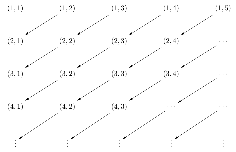
The idea is to define the diagonal \(k\) as \(k = x + y\) for \(k = 2, 3, \dots\). For example if \(k = 3\) then for \((1, 2)\) and \((2, 1)\) we have that \(k = 1 + 2 = 2 + 1\).
Each diagonal \(k\) has \(k-1\) elements and before the \(k\) diagonal there are \(1 + \cdots + k - 2 = \frac{(k-2)(k-1)}{2}\) elements where \(k = x + y\).
Furthermore we can fix the position of the element \((x,y)\) as \(F(x,y) = \frac{(x + y - 2)(x + y - 1)}{2} + x\). For example for the pair \((4,1)\) we have that \(F(4,1) = \frac{(4 + 1 - 2)(4 + 1 - 1)}{2} + 4 = 10\).
Corollary D.6
Proof.
Because \(A \approx \mathbb{P}\) and \(B \approx \mathbb{P}\) then by Lemma D.2 a \(A \times B \approx \mathbb{P} \times \mathbb{P}\).
Also by Theorem D.10 \(\mathbb{P} \times \mathbb{P} \approx \mathbb{P}\) so by Theorem D.1 c \(A \times B \approx \mathbb{P}\).
Because \(A^{P_n} = \{ f \mid f: P_n \longrightarrow A \}\) let proceed by induction.
Base step \((n = 1)\): If \(A^{P_1} = A^{\{ 1 \}}\). Also because \(A^{\{ 1 \}} = \{ f \mid f: \{ 1 \} \longrightarrow A \}\) then \(f \in A^{\{ 1 \}}\) if \(f(1) = a\) for some \(a \in A\). Therefore \(\Psi: A^{\{ 1 \}} \xrightarrow[onto]{1-1} A\) where \(\Psi(f) = a\) such that \(f(1) = a\).
Induction hypothesis \((n \leq k)\): \(A^{P_k} \approx A\)
Induction step \((n = k + 1)\): \(A^{P_{k+1}} = A^{P_{k} \cup \{ k + 1 \}}\). Also because \(P_{k} \cap \{ k + 1 \} = \emptyset\) by Lemma D.3 a \(A^{P_{k} \cup \{ k + 1 \}} \approx A^{P_{k}} \times A^{k+1}\).
We know by the induction hypothesis that \(A^{P_k} \approx A\). Also \(A^{k+1} \approx A\) where we can use the same proof as in the base case. Therefore by Lemma D.2 a \(A^{P_k} \times A^{k+1} \approx A \times A\). But \(A \approx \mathbb{P}\) is denumerable so by Corollary D.6 a \(A \times A \approx \mathbb{P}\). Furthermore by Theorem D.1 b and c \(A^{P_k} \times A^{k+1} \approx A\). So it must be the case that \(A^{P_{k+1}} \approx A\).
Because \(A \approx \mathbb{P}\) and \(B \approx P_n\) then by Lemma D.2 b \(A^B \approx \mathbb{P}^{P_n}\). Also by Corollary D.6 \(\mathbb{P}^{P_n} \approx \mathbb{P}\) so by Theorem D.1 c \(A^B \approx \mathbb{P}\).
Lemma D.5 If \(A\) has at least 2 elements and \(B\) has at least 2 elements then \(A \cup B \leq A \times B\)
Proof. Let \(a_1 \in A\) and \(a_2 \in A\) with \(a_1 \neq a_2\). Also let \(b_1 \in B\) and \(b_2 \in B\) with \(b_1 \neq b_2\). Define \(F: A \cup B \longrightarrow A \times B\) as follows:
\[F(u) = \begin{cases} (u, b_1) & \text{ if } u \in A \\ (a_2, b_2) & \text{ if } u = b_1 \in B - A \\ (a_1, u) & \text{ if } u \in B - A \land u \neq b_1 \end{cases}\]
Then \(F: A \cup B \xrightarrow[onto]{1-1} A \times B\).
Note: \(A\) and \(B\) need to have at least 2 elements or it is not possible to have a one-one function from \(A \cup B\) to \(A \times B\). For example, if \(A = \{ a \}\) and \(B = \{ b_1 , b_2 \}\) then \(A \cup B = \{ a, b_1, b_2 \}\) and \(A \times B = \{ (a, b_1), (a, b_2) \}\). Therefore there is no one-one function from \(A \cup B\) to \(A \times B\) because \(A \cup B \approx P_3\) and \(A \times B \approx P_2\).
Exercise D.9
If \(A\) and \(B\) are denumerable, prove that \(A \cup B\) is denumerable.
If \(A\) is denumerable and \(B\) is finite, prove that \(A \cup B\) is denumerable.
If \(A\) is a nonempty finite set of denumerable sets, prove that \(\bigcup_{B \in A} B\) is denumerable.
If \(A\) is a denumerable set of denumerable sets, prove that \(\bigcup_{B \in A} B\) is denumerable.
Solution D.9.
If \(A \approx \mathbb{P}\) and \(B \approx \mathbb{P}\) then by Theorem D.1 b \(\mathbb{P} \approx A\) and \(A \times B \approx \mathbb{P}\) by Corollary D.6 1.
Also by Lemma D.5 \(A \cup B \leq A \times B\). Therefore by Theorem D.2 b \(A \cup B \leq \mathbb{P}\).
Furthermore because \(\mathbb{P} \approx A\) then there is some \(F: \mathbb{P} \xrightarrow[onto]{1-1} A\) so we can define \(G: \mathbb{P} \xrightarrow[]{1-1} A \cup B\) such that \(G(n) = F(n)\). Therefore \(P \leq A \cup B\).
Because \(A \cup B \leq \mathbb{P}\) and \(P \leq A \cup B\) by Theorem D.4 \(A \cup B \approx \mathbb{P}\).
Let \(A \approx \mathbb{P}\) and \(B = \emptyset\) or \(B \approx P_n\).
If \(B = \emptyset\) then \(A \cup B = A\) so \(A \cup B \approx \mathbb{P}\).
If \(B \approx P_n\) and \(B \subseteq A\) then \(A \cup B = A\) so \(A \cup B \approx \mathbb{P}\)
If \(B \approx P_n\) and \(B \not \subseteq A\) let \(B^* = B - A\) where \(B^* = \emptyset\) or \(B^* \neq \emptyset\) then \(B^*\) is finite by Theorem D.6 because b \(B^* \subseteq B\), so \(B^* \approx P_k\). So \(A \cup B = A \cup (B - A) = A \cup B^*\). Because \(F: A \xrightarrow[onto]{1-1} \mathbb{P}\) and \(G: B^* \xrightarrow[onto]{1-1} P_k\) then we can define:
\[\Psi(u) = \begin{cases} G(u) & \text{ if } u \in B^* \\ F(u) + k & \text{ if } u \in A \end{cases}\]
Where \(\Psi: A \cup B \xrightarrow[onto]{1-1} \mathbb{P}\)
We can use Definition 2.1 iii because \(A\) is a nonempty finite set of denumerable sets.
Base step \((n = 1)\): Then \(A = \{ A_1 \}\) where \(A_1\) is a denumerable set. Therefore \(\bigcup_{B \in A} B = A_1\) so \(\bigcup_{B \in A}\) is denumerable.
Induction hypothesis \((n \leq k)\): If \(A = \{ A_1, \ldots, A_k \}\) then \(\bigcup_{B \in A} B\) is denumerable.
Induction step \((n = k + 1)\): Let \(A = \{ A_1, \ldots, A_k, A_{k+1} \}\) then \(A = A^* \cup \{ A_{k+1} \}\) where \(A = \{ A_1, \ldots, A_k \}\). By the induction hypothesis \(\bigcup_{B \in A^*} B\) is denumerable and also by assumpytion \(A_{k+1}\) is also denumerable. Therefore by Exercise D.9 1 \(\left( \bigcup_{B \in A^*} B \right) \cup A_{k+1} = \bigcup_{B \in A} B\) is also denumerable.
By Definition 2.1 iii we have that \(\bigcup_{B \in A} B\) is denumerable if \(A\) is a non empty finite set of denumerable sets.
In this case we can not apply Definition 2.1 iii because \(A = \{ A_1, \ldots, A_n, \ldots \}\). Therefore \(\mathscr{K}(A) = \mathscr{K}(\mathbb{P})\) where \(\mathscr{K}(\mathbb{P}) \not \in \mathbb{P}\).
However, we have that for each \(A_i \in A\) it exists \(F_i\) such that \(F_i: A_i \xrightarrow[onto]{1-1} \mathbb{P}\).
Let’s assume first that \(\bigcap_{A_i \in A} A_i = \emptyset\). Then we can thing of each element of \(\bigcup_{A_i \in A} A_i\) as a grid such that:
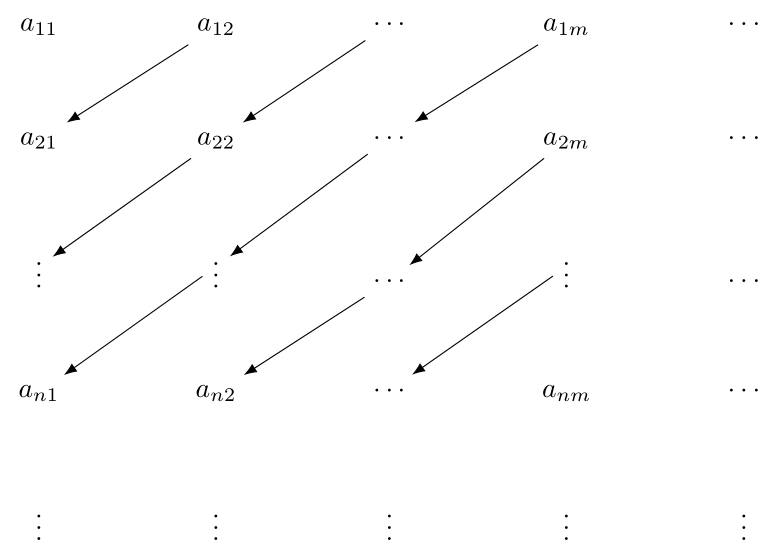
Where \(a_{ij} \in A_i\). By Theorem D.10 let \(G: \mathbb{P} \times \mathbb{P} \xrightarrow[onto]{1-1} \mathbb{P}\) such that \(G(n,m) = \frac{(n + m - 2)(n + m - 1)}{2} + n\). Therefore we can define \(\Psi: \bigcup_{A_i \in A} (\{ i \} \times A_i) \xrightarrow[onto]{1-1} \mathbb{P}\) such that \(\Psi(i, a) = G(i, F_i(a))\) where \(a \in A_i\).
Now assume \(\bigcap_{A_i \in A} A_i \neq \emptyset\), so at least one element could appear in more than one set in \(A\). We can define a one-one function from \(\bigcup_{A_i \in A} A_i\) into the disjoint union \(\bigsqcup_{A_i \in A} A_i = \bigcup_{A_i \in A} (\{ i \} \times A_i)\) such that \(H: \bigcup_{A_i \in A} A_i \xrightarrow[]{1-1} \bigsqcup_{A_i \in A} A_i\) where:
For each element \(x \in \bigsqcup_{A_i \in A} A_i\), pick \(i \in \mathbb{P}\) such that \(x \in A_i\)
Then assign \(x\) to \((i, x) \in \{ i \} \times A_i\)
Therefore by Theorem 1.14 \(\Psi \circ H: \bigcup_{A_i \in A} A_i \xrightarrow[]{1-1} \mathbb{P}\). So \(\bigcup_{A_i \in A} A_i \leq \mathbb{P}\).
Furthermore, let’s \(M: \mathbb{P} \xrightarrow[]{1-1} \bigcup_{A_i \in A} A_i\) such that \(M(i) = a_i\) where \(a_i \in A_i\). So \(\mathbb{P} \leq \bigcup_{A_i \in A} A_i\).
Finally by Theorem D.4 \(\bigcup_{A_i \in A} A_i \approx \mathbb{P}\).
Theorem D.11 The following sets are denumerable:
Proof.
We can build \(F\) such that \(F: \mathbb{P} \xrightarrow[onto]{1-1} \mathbb{Z}\) where:
\[F(p) = \begin{cases} 0 & \text{ if } p = 1 \\ \frac{p}{2} & \text{ if } p = 2k \\ -\frac{p-1}{2} & \text{ if } p = 2k + 1 \end{cases}\]
In code using the R programming language:
p_to_z <- function(p) {
if (p == 1) {
z = 0
} else if (p %% 2 == 0) {
z = p / 2
} else {
z = -((p - 1) / 2)
}
return(z)
}
# Test with p = 9
p_to_z(p = 9)[1] -4For this proof check out (Aigner and Ziegler 2018, chap. 19) which explains the Calkin–Wilf listing. Create the following tree (See Figure D.5):
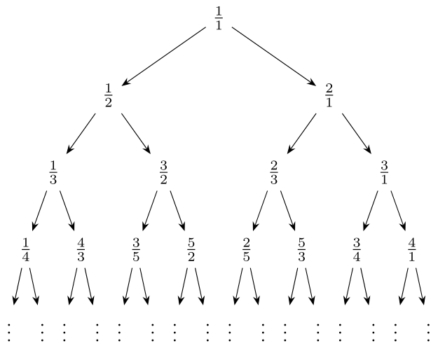
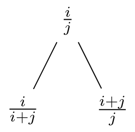
Where \(\frac{1}{1}\) is at the top of the tree and every node \(\frac{i}{j}\) has 2 sons:
Therefore we can generate the list \(\frac{1}{1}, \frac{1}{2}, \frac{2}{1}, \frac{1}{3}, \frac{3}{2}, \frac{2}{3}, \frac{3}{1}, \frac{1}{4}, \frac{4}{3}, \frac{3}{5}, \frac{5}{2}, \frac{2}{5}, \frac{5}{3}, \frac{3}{4}, \frac{4}{1} \ldots\)
Also we have the following properties:
All fractions in the tree are reduced, that is if \(gcd(i, j) = 1\) then \(gcd(i, i + j) = 1\) and \(gcd(i + j, j) = 1\) where \(gcd\) is the greatest common divisor and is defined as \(gcd(i,j) = max\{ d \in \mathbb{Z}_{>0} \mid d | i \land d | j \}\)
Every reduced fraction appears at least once. If \(\frac{i}{j} \neq 1\) then \(i > j\) or \(i < j\).
Therefore, by applying this rule leads as back to \(\frac{1}{1}\). This provides a unique finite path back to the root.
Every reduced fraction appears exactly once. If \(\frac{i}{j} \neq 1\) then \(i > j\) or \(i < j\). Therefore \(\frac{i}{j}\) can only have one unique parent:
So we can obtain the sequence using Figure D.5 by starting at the root and then visiting all nodes at each level from left to right:
\[\frac{1}{1}, \frac{1}{2}, \frac{2}{1}, \frac{1}{3}, \frac{3}{2}, \frac{2}{3}, \frac{3}{1}, \frac{1}{4}, \frac{4}{3}, \frac{3}{5}, \frac{5}{2}, \frac{2}{5}, \frac{5}{3}, \frac{3}{4}, \frac{4}{1}, \ldots\]
The denominator of the \(n\)-th fraction equals the numerator of the \(n+1\)-th fraction in the above list.
It is true for the first and second position in the list
If \(\frac{i}{j}\) is a left son the father is \(\frac{i}{j-i}\) and the right son is \(\frac{j}{j-i}\)
If \(\frac{i}{j}\) is a right son and at the right boundary then \(j=1\) and the next fraction in the list is at the left boundary where the numerator is \(1\)
If \(\frac{i}{j}\) is a right son and at the interior where the next fraction is \(\frac{i^{'}}{j^{'}}\) then the father of \(\frac{i}{j}\) is \(\frac{i-j}{j}\) and the father of \(\frac{i^{'}}{j^{'}}\) is \(\frac{i^{'}}{j^{'}-i^{'}}\).
But how we can obtain a function \(S(y)\) as described in Definition 2.1 where \(y \in \mathbb{Q}_{>0}\)?
In our tree we have that:
If \(x = \frac{i}{j}\) then \(x + 1 = \frac{i+j}{j}\). Also \(x + 1 = \frac{\frac{i+j}{i}}{\frac{j}{i}} = \frac{\frac{i+j}{i}}{\frac{1}{x}}\) so \(\frac{x+1}{x} = \frac{i+j}{i}\) and \(\frac{x}{x+1} = \frac{i}{i+j}\).
Therefore we have that:
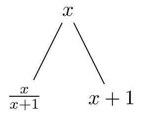
In that way we can expand the tree to identify which is the next fraction in the list in the following way for the \(k\) level:
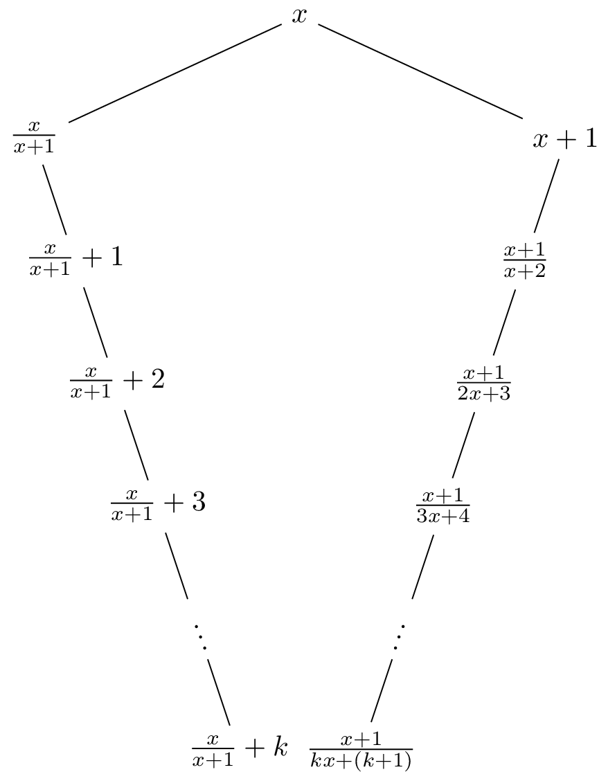
Therefore, if \(y = \frac{x}{x+1} + k\) then \(k = \left\lfloor y \right\rfloor\) is the integral part of \(y\) and \(\frac{x}{x+1} = \{y\}\) is fractional part of \(y\) where \(y = \{y\} + \left\lfloor y \right\rfloor\).
So \(\frac{x + 1}{kx + (k+1)} = \frac{x + 1}{1 + k(x+1)} = \frac{1}{\frac{1}{x+1} + k} = \frac{1}{1 - \frac{x}{x+1} + k} = \frac{1}{1 - \{y\} + \left\lfloor y \right\rfloor}\).
This means that \(S(y) = \frac{1}{1 - \{y\} + \left\lfloor y \right\rfloor} = \frac{1}{2\left\lfloor y \right\rfloor - y + 1}\) or alternatively \(y_1 = \frac{1}{1}\) and \(y_{n+1} = \frac{1}{2\left\lfloor y_n \right\rfloor - y_n + 1}\).
Now, how you can obtain the position \(k\) in the list using the Calkin–Wilf tree?
Think of each branch as left \((0)\) or right \((1)\) where the root, \(\frac{1}{1}\), is associated with \(1\). So for example to reach \(\frac{5}{2}\) we can represent it as \(RLRR\) or \(1011\) where \(\frac{5}{2}\) is in the position \(11\) in the tree and the representation of \(11\) in base 2 is \(1011\)
So the function will be as follows:
Where, \(0 < n \leq k\), \(r_{n-1} = \frac{i}{j}\), \(k_2\) is the binary representation of \(k\) and \(k_2(n)\) is the \(n\) element from left to right in the binary representation of \(k\).
For example let \(k = 4\) and \(n = 2\). So \(4_2 = 100\), \(k_4(2) = 0\) and \(r_2 = \frac{1}{2}\) where \(r_1 = \frac{1}{1}\). In that way if you want to know \(r_4\) you use \(r_0\) to calculate \(r_1\), \(r_1\) to calculate \(r_2\), \(r_2\) to calculate \(r_3\) and \(r_3\) to finally calculate \(r_4\).
In Listing D.2 it is pointed out a possible way to find the \(k\) position in the Calkin–Wilf tree using the R programming language.
p_to_q_positive <- function(p) {

# Function to find the binary representation
decimal_to_binary <- function(decimal_num) {

  binary_num <- integer(0)

  while (decimal_num > 0) {
  remainder <- decimal_num %% 2
  binary_num <- c(remainder, binary_num) # Add at the beginning
  decimal_num <- decimal_num %/% 2

  }

  return(binary_num)

 }

 # Binary representation of the position
 position_to_binary <- decimal_to_binary(decimal_num = p)
 # Root
 frac <- c(0,1)

 for (i in position_to_binary) {

   if (i == 0) {
   frac[2] <- frac[1] + frac[2]
   } else {
     frac[1] <- frac[1] + frac[2]
   }

  }

 return(frac)

 }

 # Test with k=4
 p_to_q_positive(p = 4)
[1] 1 3By thm-denumerable-sets b. let \(\Phi\) be a one-one correspondence between \(\mathbb{Q}^+\) and \(\mathbb{P}\). Then define:
\[\Psi(z) = \begin{cases} \Phi(z) & \text{ if } z \in \mathbb{Z}^+ \\ 0 & \text{ if } z = 0 \\ -\Phi(-z) & \text{ if } -z \in \mathbb{Z}^+ \end{cases}\]
Then \(\Psi: \mathbb{Z} \xrightarrow[onto]{1-1} \mathbb{Q}\). In code using the R programming language:
z_to_q <- function(z) {

 if (z > 0) {
   r = p_to_q_positive(p = z)
  } else if (z < 0) {
   r = p_to_q_positive(p = -z)
   r[1] = -r[1]
  } else {
   r = 0
  }

  return(r)

}

# Test with z=-4
z_to_q(z = -4)
[1] -1 3But by Theorem D.11 a. \(\mathbb{P} \approx \mathbb{Z}\). Hence, \(\mathbb{P} \approx \mathbb{Q}\). In code using the R programming language:
# Test with p = 9
9 |>
 p_to_z() |>
 z_to_q()
[1] -1 3The cardinal number \(\mathscr{K}(\mathbb{P})\) is traditionally denoted by \(\aleph_0\). Thus, all denumerable sets have cardinal numbers \(\aleph_0\).
By Exercise D.8 the only cardinal numbers smaller than \(\aleph_0\) are the finite cardinal numbers.
By Exercise D.4 1. \(\aleph_0\) is the smallest infinite cardinal number.
By Theorem D.3 the cardinal number of \(\mathscr{P}(\mathbb{P})\) is bigger that \(\aleph_0\)
Let \(\mathbb{R}\) denote the set of real numbers.
Theorem D.12 The half-open interval \([0,1) = \{x \mid x \in \mathbb{R} \land 0 \leq x < 1 \}\) is not denumerable.
Proof. Assume that \([0,1)\) is denumerable. Let \(\Psi: \mathbb{P} \xrightarrow[onto]{1-1} [0,1)\). Denote \(\Psi(n) = r_n\) for each \(n \in \mathbb{P}\). Each \(r_n\) can be represented by an infinite decimal \(.a_{n1}a_{n2}a_{n3}\ldots\) where \(a_{nm} \in \{ 0, 1, \ldots, 9 \}\) and \(m \in \mathbb{P}\).
Also because infinite decimals with an infinite tail of \(9\)’s, such as \(0.427999\ldots\), represent the same number as another decimal with an infinite tail of \(0\)’s, in the example \(0.248000\ldots\), we avoid decimal expansions that terminate in repeating \(9\)’s.
So we have that:
\[\begin{align*} r_1 & = \; .a_{11}a_{12}a_{13}\ldots \\ r_2 & = \; .a_{21}a_{22}a_{23}\ldots \\ r_3 & = \; .a_{31}a_{32}a_{33}\ldots \\ & \;\; \vdots \end{align*}\]
Now, define a new decimal \(.c_1c_2c_3\ldots\) such that:
\[c_n = \begin{cases} 0 & \text{ if } a_{nn} \neq 0 \\ 1 & \text{ if } a_{nn} = 0 \end{cases}\]
Then the decimal \(.c_1c_2c_3\ldots\) differs from each decimal \(r_n\) in the \(n\)-th place. Hence, \(.c_1c_2c_3\ldots\) does not appear in the list, contradicting the assumption that \(\Psi: \mathbb{P} \xrightarrow[onto]{1-1} [0,1)\).
By a generalized interval, we shall mean a set of real numbers of nay of the following forms:
\[\begin{align*} [a,b] & = \{ x \in \mathbb{R} \mid a \leq x \leq b \} \\ (a,b) & = \{ x \in \mathbb{R} \mid a < x < b \} \\ [a,b) & = \{ x \in \mathbb{R} \mid a \leq x < b \} \\ (a,b] & = \{ x \in \mathbb{R} \mid a < x \leq b \} \\ [a,\infty) & = \{ x \in \mathbb{R} \mid a \leq x \} \\ (a,\infty) & = \{ x \in \mathbb{R} \mid a < x \} \\ (-\infty, a] & = \{ x \in \mathbb{R} \mid x \leq a \} \\ (-\infty, a) & = \{ x \in \mathbb{R} \mid x < a \} \end{align*}\]
Theorem D.13 All generalized intervals are equinumerous with each other and with the whole set \(\mathbb{R}\) of real numbers.
Proof.
First, we map \((a, b)\) into \((c, d)\).
To do that we map \((a, b)\) into \((0, 1)\). Take \(x \in (a, b)\) and shift \(x\) to the left by \(a\) applying \(x - a\) and then scale it by \(b - a\) such that \(\frac{x - a}{b - a}\):
\[\begin{align*} a & < x < b \\ 0 & < x - a < b - a \\ 0 & < \frac{x - a}{b-a} < 1 \end{align*}\]
Then scale by the interval length \(d-c\) and shift to the starting point \(c\):
\[\begin{align*} 0 & < \frac{x - a}{b-a} < 1 \\ 0 & < (d-c)\frac{x - a}{b-a} < d-c \\ c & < (d-c)\frac{x - a}{b-a} + c < d \\ \end{align*}\]
So an specific bijection between \((a,b)\) and \((c,d)\) is \((d-c)\frac{x - a}{b-a} + c\). Therefore \((a,b) \approx (c,d)\).
Second, we map \((0, 1)\) into \((0, \infty)\) in the following way:
\[\begin{align*} 0 & < x < 1 \\ -1 & < -x < 0 \\ 0 & < 1-x < 1 \\ 1 & < \frac{1}{1-x} \\ 0 & < \frac{1}{1-x} - 1 \end{align*}\]
Therefore \(\frac{1}{1-x} - 1 \in (0, \infty)\) and \((0, 1) \approx (0, \infty)\) where the explicity bijection is \(\frac{1}{1-x} - 1\).
Furthermore, we can map \((0, 1)\) into \((a, \infty)\) with \(\frac{1}{1-x} - 1 + a\).
Also, we can map \((0, 1)\) into \((-\infty, 0)\) with:
\[\begin{align*} 0 & < \frac{1}{1-x} - 1 \\ 0 & > -\left( \frac{1}{1-x} - 1 \right) \end{align*}\]
So, we can map \((0, 1)\) into \((-\infty, a)\) with \(-\left( \frac{1}{1-x} - 1 \right) + a\).
Third, we map \((-1, 1)\) into \(\mathbb{R}\) in the following way:
\[\Psi(u) = \begin{cases} \frac{1}{1-x} - 1 & \text{ if } u \in (0,1) \\ 0 & \text{ if } u = 0 \\ -\frac{1}{1-(-x)} - 1 & \text{ if } u \in (-1,0) \end{cases}\]
Therefore, \((-1,1) \approx \mathbb{R}\).
Now, assume \(I\) is a generalized interval. So, there is some interval \((a,b)\) included in \(I\) such that \((a,b) \subseteq I\).
By the above results \((a,b) \approx (-1,1)\) so \((-1,1) \leq I\). Also because \(\mathbb{R} \approx (-1,1)\) then \(\mathbb{R} \leq I\).
Converserly, because \(I \subseteq \mathbb{R}\) then \(I \leq \mathbb{R}\)
By Theorem D.4 \(I \approx \mathbb{R}\).
Exercise D.10
Solution D.10. Because \(A \subseteq \mathbb{R}\) then \(A \leq \mathbb{R}\).
Because \(I \subseteq A\) then \(I \leq A\). Also \(\mathbb{R} \approx I\) so \(\mathbb{R} \leq A\).
By Theorem D.4 \(A \approx \mathbb{R}\).
The symbol \(\mathfrak{c}\) is used to denote \(\mathscr{K}(\mathbb{R})\), the cardinal number of \(\mathbb{R}\). \(\mathfrak{c}\) is called the power of continuum.
From Theorem D.13 all generalized intervals have cardinal number \(\mathfrak{c}\).
From Theorem D.12 \(\aleph_0 <_K \mathfrak{c}\).
Whether there is a cardinal number between \(\aleph_0\) and \(\mathfrak{c}\) is a long-standing mathematical problem called the continuum hypothesis.
The fact proved in Theorem D.12 that \(\mathbb{P} < \mathbb{R}\) is not new. By Theorem D.3 \(\mathbb{P} < \mathscr{P}(\mathbb{P})\) and the following theorem tell us that this result is equivalent to \(\mathbb{P} < \mathbb{R}\).
Theorem D.14 \(\mathbb{R} \approx \mathscr{P}(\mathbb{P})\). That is the set of real numbers is equinumerous with the set of all sets of positive numbers.
Proof. By Theorem D.9 \(\{ 0, 1 \}^{\mathbb{P}} \approx \mathscr{P}(\mathbb{P})\).
Hence we can prove that \(\mathbb{R} \approx \{ 0, 1 \}^{\mathbb{P}}\).
Since \(\mathbb{R} \approx [0,1)\) by Theorem D.13, it suffices to prove that \([0,1) \approx \{ 0, 1 \}^{\mathbb{P}}\).
Any number in \([0,1)\) has an infinite binary expansion just as it has an infinite decimal representation. In the case of 2 binary representations for the same number, we discard the representation with an infinite tail of \(1\)’s.
Every infinite binary (See Appendix H) representation can be considered to be an element of \(\{ 0, 1\}^{\mathbb{P}} = \{ f \mid f: \mathbb{P} \longrightarrow \{ 0, 1\} \}\). For example \(0.5\) in base \(10\), \((0.5)_{10}\), can be represented in base \(2\) as \(0.1000\ldots\), \((0.1000\ldots)_2\), where it has an associated \(f: \mathbb{P} \longrightarrow \{ 0, 1\}\) such that \(1 = f(1), 0 = f(2), 0 = f(3), 0 = f(4), \ldots\). Thus, we have a one-one correspondence between \([0, 1)\) and a subset of \(\{ 0, 1\}^{\mathbb{P}}\) because those binary representations with infinite tails of \(1\)’s were not used. For example \(0.4999\ldots\) in base \(10\), \((0.4999\ldots)_{10}\), represented in base \(2\) as \(0.0111\ldots\), \((0.0111\ldots)_2\), is not considered. Therefore, that range of this one-one correspondence is not equal to the range of \(\{ 0, 1\}^{\mathbb{P}}\). So, \(G: [0,1) \xrightarrow[]{1-1} \{ 0, 1 \}^{\mathbb{P}}\) and \([0,1) \leq \{ 0, 1 \}^{\mathbb{P}}\).
Conversely, let’s represent the numbers in \([0,1)\) in base \(3\). So, for example \(0.5\) in base \(10\), \((0.5)_{10}\),is represented as \(0.111\ldots\) in base \(3\), \((0.111\ldots)_{3}\) and \(0.1\) in base \(10\), \((0.1)_{10}\),is represented as \(00220022\ldots\) in base \(3\), \(00220022\ldots)_{3}\). Then with each element \(g\) in \(\{ 0, 1\}^{\mathbb{P}}\) we associate the real number in \([0,1)\) the base \(3\) representation provided by \(0.g(1)g(2)\ldots\) where \(g(i) \neq 2\). So, \(H: \{ 0, 1 \}^{\mathbb{P}} \xrightarrow[]{1-1} [0,1)\) taking into account that numbers like \(0.1\) represented in base \(3\) as \(00220022\ldots)_{3}\) are not part of the range of this one-one correspondence. Therefore, \([0,1) \geq \{ 0, 1 \}^{\mathbb{P}}\).
Because, \([0,1) \leq \{ 0, 1 \}^{\mathbb{P}}\) and \([0,1) \geq \{ 0, 1 \}^{\mathbb{P}}\) then by Theorem D.4 \([0,1) \approx \{ 0, 1 \}^{\mathbb{P}}\).
Lemma D.6 For any sets \(A\) and \(B\), there exist sets \(A_1\), \(B_1\) such that \(A_1 \approx A\), \(B_1 \approx B\) and \(A_1 \cap B_1 = \emptyset\).
Proof. Let \(A_1 = A \times \{ 0 \}\) and \(B_1 = B \times \{ 1 \}\). Then \(F(a) = (a, 0)\), \(G(b) = (b, 0)\) so \(F: A \xrightarrow[onto]{1-1} A_1\) and \(G: B \xrightarrow[onto]{1-1} B_1\) and \(A_1 \cap B_1\). Therefore, \(A_1 \approx A\) and \(B_1 \approx B\).
Definition D.6 (Addition) Let \(\mathfrak{m}\) and \(\mathfrak{n}\) be cardinal numbers. Take any sets \(A\), \(B\) such that \(\mathscr{K}(A) = \mathfrak{m}\), \(\mathscr{K}(B) = \mathfrak{n}\) and \(A \cap B = \emptyset\). Then
\[\mathfrak{m} + \mathfrak{n} = \mathscr{K}(A \cup B)\] Note: By Lemma D.2 c, the result \(\mathfrak{m} + \mathfrak{n}\) does not depend upon the choice of \(A\) and \(B\).
Also the condition \(A \cap B = \emptyset\) is important. For example, if \(A = \{ 1, 2, 3 \}\) and \(B = \{ 3, 4 \}\) then \(\mathscr{K}(A) = 3\), \(\mathscr{K}(B) = 2\), \(\mathscr{K}(A \cup B) = 3\) where \(\mathscr{K}(A) + \mathscr{K}(B) = 5 > \mathscr{K}(A \cup B) = 3\).
Definition D.7 (Multiplication and Exponentiation) Let \(\mathfrak{m}\) and \(\mathfrak{n}\) be cardinal numbers, and let \(A\), \(B\) be any sets such that \(\mathscr{K}(A) = \mathfrak{m}\), \(\mathscr{K}(B) = \mathfrak{n}\). Then
\[\mathfrak{m} \times \mathfrak{n} = \mathscr{K}(A \times B),\]
and
\[\mathfrak{m}^{\mathfrak{n}} = \mathscr{K}(A^B).\] By Lemma D.2 a, b we know that \(\mathfrak{m} \times \mathfrak{n}\) and \(\mathfrak{m}^{\mathfrak{n}}\) do not depend upon the choice of \(A\) and \(B\).
Theorem D.15
\(\mathfrak{m} + \mathfrak{n} = \mathfrak{n} + \mathfrak{m}\)
\(\mathfrak{m} + (\mathfrak{n} + \mathfrak{p}) = (\mathfrak{m} + \mathfrak{n}) + \mathfrak{p}\)
\(\mathfrak{m} + 0 = \mathfrak{m}\) (Remember that \(\mathscr{K}(\emptyset) = 0\))
\(\mathfrak{m} \times \mathfrak{n} = \mathfrak{n} \times \mathfrak{m}\)
\(\mathfrak{m} \times (\mathfrak{n} \times \mathfrak{p}) = (\mathfrak{m} \times \mathfrak{n}) \times \mathfrak{p}\)
\(\mathfrak{m} \times 1 = \mathfrak{m}\) (Remember that \(\mathscr{K}(P_1)\))
\(\mathfrak{m} \times (\mathfrak{n} + \mathfrak{p}) = (\mathfrak{m} \times \mathfrak{n}) + (\mathfrak{m} + \mathfrak{p})\)
\(\mathfrak{m}^0 = 1\)
\(\mathfrak{n} \neq 0 \Longrightarrow 0^{\mathfrak{n}} = 0\)
\(\mathfrak{m}^{\mathfrak{n} + \mathfrak{p}} = \mathfrak{m}^{\mathfrak{n}} \times \mathfrak{m}^{\mathfrak{p}}\)
\((\mathfrak{m}^{\mathfrak{n}})^{\mathfrak{p}} = \mathfrak{\mathfrak{m}^{\mathfrak{n} \times \mathfrak{p}}}\)
\(2 \leq_K \mathfrak{m} \land 2 \leq_K \mathfrak{n} \Longrightarrow \mathfrak{m} + \mathfrak{n} \leq_K \mathfrak{m} \times \mathfrak{n}\)
Proof. Let \(\mathscr{K}(A) = \mathfrak{m}\), \(\mathscr{K}(B) = \mathfrak{n}\) and \(\mathscr{K}(C) = \mathfrak{p}\) where \(A \cap B = \emptyset\), \(A \cap C = \emptyset\), \(B \cap C = \emptyset\) and \(A \cap P_1 = \emptyset\):
\(\begin{aligned} \mathfrak{m} + \mathfrak{n} & = \mathscr{K}(A \cup B) \\ & = \mathscr{K}(B \cup A); A \cup B = B \cup A \\ & = \mathfrak{n} + \mathfrak{m} \end{aligned}\)
\(\begin{aligned} \mathfrak{m} + (\mathfrak{n} + \mathfrak{p}) & = \mathscr{K}(A \cup (B \cup C)) \\ & = \mathscr{K}((A \cup B) \cup C)); A \cup (B \cup C) = (A \cup B) \cup C) \\ & = (\mathfrak{n} + \mathfrak{m}) + \mathfrak{p} \end{aligned}\)
\(\begin{aligned} \mathfrak{m} + 0 & = \mathscr{K}(A \cup \emptyset); A \cap \emptyset \\ & = \mathscr{K}(A); A \cup \emptyset = A \\ & = \mathfrak{m} \end{aligned}\)
\(\begin{aligned} \mathfrak{m} \times \mathfrak{n} & = \mathscr{K}(A \times B) \\ & = \mathscr{K}(B \times A); A \times B \approx B \times A \\ & = \mathfrak{n} \times \mathfrak{m} \end{aligned}\)
\(\begin{aligned} \mathfrak{m} \times (\mathfrak{n} \times \mathfrak{p}) & = \mathscr{K}(A \times (B \times C)) \\ & = \mathscr{K}((A \times B) \times C); A \times (B \times C) \approx (A \times B) \times C \\ & = (\mathfrak{n} \times \mathfrak{m}) \times \mathfrak{p} \end{aligned}\)
\(\begin{aligned} \mathfrak{m} \times 1 & = \mathscr{K}(A \times P_1) \\ & = \mathscr{K}(A); A \approx A \times P_1 \\ & = \mathfrak{m} \end{aligned}\)
\(\begin{aligned} \mathfrak{m} \times (\mathfrak{n} + \mathfrak{p}) & = \mathscr{K}(A \times (B \cup C)) \\ & = \mathscr{K}((A \times B) \cup (A \times C)); A \times (B \cup C) = A \times B \cup A \times C) \\ & = (\mathfrak{m} \times \mathfrak{n}) + (\mathfrak{m} \times \mathfrak{p}) \end{aligned}\)
\(\begin{aligned} \mathfrak{m}^0 & = \mathscr{K}(A^{\emptyset}) \\ & = \mathscr{K}(\{ \emptyset \}); A^{\emptyset} = \{ \emptyset \} \\ & = 1 \end{aligned}\)
Let \(\mathfrak{n} \neq 0\) then \(0^{\mathfrak{n}} = \mathscr{K}(\emptyset^B)\) where \(B \neq \emptyset\). Because \(\emptyset^B = \{ f \mid f: B \longrightarrow \emptyset \}\), but by Definition 1.58 \(f\) is not a function. Therefore, \(\emptyset^B = \emptyset\). So, \(\mathscr{K}(\emptyset^B) = \mathscr{K}(\emptyset) = 0\) and \(0^{\mathfrak{n}} = 0\) when \(\mathfrak{n} \neq 0\).
\(\begin{aligned} \mathfrak{m}^{\mathfrak{n} + \mathfrak{p}} & = \mathscr{K}(A^{B \cup C}) \\ & = \mathscr{K}(A^B \times A^C); A^{B \cup C} \approx A^B \times A^C \text{ when } B \cap C = \emptyset \\ & = \mathfrak{m}^{\mathfrak{n}} \times \mathfrak{m}^{\mathfrak{p}} \end{aligned}\)
\(\begin{aligned} (\mathfrak{m}^{\mathfrak{n}})^{\mathfrak{p}} & = \mathscr{K}((A^B)^C) \\ & = \mathscr{K}(A^{B \times C}); (A^B)^C \approx A^{B \times C} \\ & = \mathfrak{m}^{\mathfrak{n} \times \mathfrak{p}} \end{aligned}\)
\(\begin{aligned} \mathfrak{m} + \mathfrak{n} & = \mathscr{K}(A \cup B) \\ & \iff A \cup B \leq A \times B \text{ if } 2 \leq_K \mathfrak{m} \land 2 \leq_K \mathfrak{n} \\ & \iff \mathscr{K}(A \cup B) \leq \mathscr{K}(A \times B) \\ & \iff \mathfrak{m} + \mathfrak{n} \leq_K \mathfrak{m} \times \mathfrak{n} \end{aligned}\)
Exercise D.11 Assume \(\mathfrak{m} \leq_K \mathfrak{n}\) and \(\mathfrak{p} \leq_K \mathfrak{q}\). Prove:
\(\mathfrak{m} + \mathfrak{p} \leq_K \mathfrak{n} + \mathfrak{q}\)
\(\mathfrak{m} \times \mathfrak{p} \leq_K \mathfrak{n} \times \mathfrak{q}\)
\(\mathfrak{m} + (\mathfrak{n} + \mathfrak{p}) >_K 0 \Longrightarrow \mathfrak{m}^{\mathfrak{p}} \leq_K \mathfrak{n}^{\mathfrak{q}}\)
Solution D.11. Also assume \(\mathscr{K}(A) = \mathfrak{m}\), \(\mathscr{K}(B) = \mathfrak{n}\), \(\mathscr{K}(C) = \mathfrak{p}\), \(\mathscr{K}(D) = \mathfrak{q}\) where \(A \cap C = \emptyset\), \(B \cap D = \emptyset\) and \((A \cap C) \cap B = \emptyset\):
\(\begin{aligned} \mathfrak{m} \leq_K \mathfrak{n} \land \mathfrak{p} \leq_K \mathfrak{q} & \iff A \leq B \land C \leq D \\ & \Longrightarrow A \cup C \leq B \cup D; \text{ where } B \cap D = \emptyset \\ & \iff \mathscr{K}(A \cup C) \leq_K \mathscr{K}(B \cup D) \\ & \iff \mathfrak{m} + \mathfrak{p} \leq_K \mathfrak{n} + \mathfrak{q} \end{aligned}\)
\(\begin{aligned} \mathfrak{m} \leq_K \mathfrak{n} \land \mathfrak{p} \leq_K \mathfrak{q} & \iff A \leq B \land C \leq D \\ & \Longrightarrow A \times C \leq B \times D \\ & \iff \mathscr{K}(A \times C) \leq_K \mathscr{K}(B \times D) \\ & \iff \mathfrak{m} \times \mathfrak{p} \leq_K \mathfrak{n} \times \mathfrak{q} \end{aligned}\)
\(\begin{aligned} \mathfrak{m} + (\mathfrak{n} + \mathfrak{p}) >_K 0 & \iff \mathscr{K}(A \cup (B \cup C)) >_K \mathscr{K}(\emptyset) \\ & \iff A \cup (B \cup C) > \emptyset \\ & \Longrightarrow A \cup (B \cup C) \neq \emptyset \\ & \Longrightarrow A^C \leq B^D \\ & \iff \mathscr{K}(A^C) \leq_K \mathscr{K}(B^D) \\ & \iff \mathfrak{m}^{\mathfrak{p}} \leq_K \mathfrak{n}^{\mathfrak{q}} \end{aligned}\)
Theorem D.16
\(\aleph_0 \times \aleph_0 = \aleph_0\)
If \(n\) is a positive integer, \(\aleph_0^n = \aleph_0\)
\(0 <_K \mathfrak{m} \leq_K \aleph_0 \Longrightarrow \mathfrak{m} \times \aleph_0 = \aleph_0\)
\(\aleph_0 + \aleph_0 = \aleph_0\)
\(\mathfrak{m} \leq_K \aleph_0 \Longrightarrow \mathfrak{m} + \aleph_0 = \aleph_0\)
Proof. Assume \(\mathscr{K}(A) = \mathfrak{m}\) where \(\mathfrak{m} \leq_K \aleph_0\):
\(\begin{aligned} \aleph_0 \times \aleph_0 & = \mathscr{K}(\mathbb{P} \times \mathbb{P}) \\ & = \mathscr{K}(\mathbb{P}); \mathbb{P} \times \mathbb{P} \approx \mathbb{P} \\ & = \aleph_0 \end{aligned}\)
\(\begin{aligned} \aleph_0^n & = \mathscr{K}(\mathbb{P}^{P_n}) \\ & = \mathscr{K}(\mathbb{P}); \mathbb{P}^{P_n} \approx \mathbb{P} \\ & = \aleph_0 \end{aligned}\)
\(\begin{aligned} 0 <_K \mathfrak{m} \land \mathfrak{m} \leq_K \aleph_0 & \Longrightarrow 1 \leq_K \mathfrak{m} \land \mathfrak{m} \leq_K \aleph_0 \\ & \Longrightarrow 1 \times \aleph_0 \leq_K \mathfrak{m} \times \aleph_0 \land \mathfrak{m} \times \aleph_0 \leq_K \aleph_0 \times \aleph_0 \\ & \iff \aleph_0 \leq_K \mathfrak{m} \times \aleph_0 \land \mathfrak{m} \times \aleph_0 \leq_K \aleph_0 \\ & \iff \mathbb{P} \leq A \times \mathbb{P} \land A \times \mathbb{P} \leq \mathbb{P} \\ & \iff \mathbb{P} \approx A \times \mathbb{P} \\ & \iff \mathscr{K}(\mathbb{P}) = \mathscr{K}(A \times \mathbb{P}) \\ & \iff \aleph_0 = \mathfrak{m} \times \aleph_0 \end{aligned}\)
\(\begin{aligned} \aleph_0 + \aleph_0 & = \mathscr{K}(\mathbb{P}) + \mathscr{K}(\mathbb{P}) \\ & = \mathscr{K}(\mathbb{P} \times \{0\}) + \mathscr{K}(\mathbb{P} \times \{1\}); \mathbb{P} \times \{0\} \approx \mathbb{P} \text{ and } \mathbb{P} \times \{1\} \approx \mathbb{P} \\ & = \mathscr{K}((\mathbb{P} \times \{0\}) \cup (\mathbb{P} \times \{1\})) \\ & = \mathscr{K}(\mathbb{P}); (\mathbb{P} \times \{0\}) \cup (\mathbb{P} \times \{1\}) \approx \mathbb{P} \\ & = \aleph_0 \end{aligned}\)
\(\begin{aligned} \mathfrak{m} + \aleph_0 & = \mathscr{K}(A) + \mathscr{K}(\mathbb{P}) \\ & = \mathscr{K}(A \times \{0\}) + \mathscr{K}(\mathbb{P} \times \{1\}); A \times \{0\} \approx A \land \mathbb{P} \times \{1\} \approx \mathbb{P} \\ & = \mathscr{K}((A \times \{0\}) \cup (\mathbb{P} \times \{1\})) \\ & = \mathscr{K}(\mathbb{P}); (A \times \{0\}) \cup (\mathbb{P} \times \{1\}) \approx \mathbb{P} \text{ and } \mathfrak{m} \leq_K \aleph_0 \text{ so } A \text{ is denumerable or finite} \\ & = \aleph_0 \end{aligned}\)
Theorem D.17
\(2^{\aleph_0} = \mathfrak{c}\)
\(\mathfrak{c} \times \mathfrak{c} = \mathfrak{c}\)
\(0 <_K \mathfrak{m} \leq_K \mathfrak{c} \Longrightarrow \mathfrak{m} \times \mathfrak{c} = \mathfrak{c}\)
\(\mathfrak{c} + \mathfrak{c} = \mathfrak{c}\)
\(\mathfrak{m} \leq_K \mathfrak{c} \Longrightarrow \mathfrak{m} + \mathfrak{c} = \mathfrak{c}\)
\(0 <_K \mathfrak{n} \leq_K \aleph_0 \Longrightarrow \mathfrak{c}^{\mathfrak{n}} = \mathfrak{c}\)
\(\mathfrak{c} <_K 2^\mathfrak{c}\)
Proof. Assume \(\mathscr{K}(A) = \mathfrak{m}\) and \(\mathscr{K}(B) = \mathfrak{n}\) where \(\mathfrak{m} \leq_K \mathfrak{c}\) and \(\mathfrak{m} \leq_K \aleph_0\):
\(\begin{aligned} 2^{\aleph_0} & = \mathscr{K}(\{0,1\}^{\mathbb{P}}) \\ & = \mathscr{K}(\mathscr{P}(\mathbb{P})); \{0,1\}^{\mathbb{P}} \approx \mathscr{P}(\mathbb{P}) \\ & = \mathscr{K}(\mathbb{R}); \mathscr{P}(\mathbb{P}) \approx \mathbb{R} \\ & = \mathfrak{c} \end{aligned}\)
\(\begin{aligned} \mathfrak{c} \times \mathfrak{c} & = 2^{\aleph_0} \times 2^{\aleph_0}; \mathfrak{c} = 2^{\aleph_0} \\ & = 2^{\aleph_0 + \aleph_0}; \mathfrak{m}^{\mathfrak{n} + \mathfrak{p}} = \mathfrak{m}^{\mathfrak{n}} \times \mathfrak{m}^{\mathfrak{p}} \\ & = 2^{\aleph_0}; \aleph_0 + \aleph_0 = \aleph_0 \\ & = \mathfrak{c}; \mathfrak{c} = 2^{\aleph_0} \end{aligned}\)
\(\begin{aligned} 0 <_K \mathfrak{m} \land \mathfrak{m} \leq_K \mathfrak{c} & \Longrightarrow 1 \leq_K \mathfrak{m} \land \mathfrak{m} \leq_K \mathfrak{c} \\ & \Longrightarrow 1 \times \mathfrak{c} \leq_K \mathfrak{m} \times \mathfrak{c} \land \mathfrak{m} \times \mathfrak{c} \leq_K \mathfrak{c} \times \mathfrak{c} \\ & \iff \mathfrak{c} \leq_K \mathfrak{m} \times \mathfrak{c} \land \mathfrak{m} \times \mathfrak{c} \leq_K \mathfrak{c} \\ & \iff \mathbb{R} \leq_K A \times \mathbb{R} \land A \times \mathbb{R} \leq_K \mathbb{R} \\ & \iff \mathbb{R} \approx A \times \mathbb{R} \\ & \iff \mathscr{K}(\mathbb{R}) = \mathscr{K}(A \times \mathbb{R}) \\ & \iff \mathfrak{c} = \mathfrak{m} \times \mathfrak{c} \\ \end{aligned}\)
Because \(0 \leq_K \mathfrak{c}\) and \(\mathfrak{c} \leq_K \mathfrak{c}\) then by Exercise D.11 1 \(\mathfrak{c} + 0 \leq_K \mathfrak{c} + \mathfrak{c}\). Therefore \(\mathfrak{c} \leq_K \mathfrak{c} + \mathfrak{c}\) by Theorem D.15 c. Using the above result:
\(\begin{aligned} \mathfrak{c} \leq_K \mathfrak{c} + \mathfrak{c} \land \mathfrak{c} + \mathfrak{c} \leq_K \mathfrak{c} \times \mathfrak{c} & \iff \mathfrak{c} \leq_K \mathfrak{c} + \mathfrak{c} \land \mathfrak{c} + \mathfrak{c} \leq_K \mathfrak{c} \\ & \iff \mathfrak{c} = \mathfrak{c} + \mathfrak{c} \end{aligned}\)
Because \(\mathfrak{c} \leq_K \mathfrak{c}\) and \(0 \leq_K \mathfrak{m}\) then by Exercise D.11 1 \(\mathfrak{c} + 0 \leq_K \mathfrak{m} + \mathfrak{c}\). Also by Theorem D.15 c \(\mathfrak{c} \leq_K \mathfrak{c} + \mathfrak{m}\). By a similar argument because \(\mathfrak{m} \leq_K \mathfrak{c}\) and \(\mathfrak{c} \leq_K \mathfrak{c}\) we have that \(\mathfrak{m} + \mathfrak{c} \leq_K \mathfrak{c} + \mathfrak{c}\). Using the above results:
\(\begin{aligned} \mathfrak{c} \leq_K \mathfrak{c} + \mathfrak{m} \land \mathfrak{m} + \mathfrak{c} \leq_K \mathfrak{c} + \mathfrak{c} & \iff \mathfrak{c} \leq_K \mathfrak{c} + \mathfrak{m} \land \mathfrak{m} + \mathfrak{c} \leq_K \mathfrak{c} \\ & \iff \mathfrak{c} \leq_K \mathfrak{m} + \mathfrak{c} \land \mathfrak{m} + \mathfrak{c} \leq_K \mathfrak{c} \\ & \iff \mathfrak{c} = \mathfrak{m} + \mathfrak{c} \end{aligned}\)
\(\begin{aligned} \mathfrak{c}^{\mathfrak{m}} & = ({2^{\aleph_0}})^{\mathfrak{m}} \\ & = 2^{\aleph_0 \times \mathfrak{m}} \\ & = 2^{\mathfrak{m} \times \aleph_0} \\ & = 2^{\aleph_0} \\ & = \mathfrak{c} \end{aligned}\)
\(\begin{aligned} \mathbb{R} < \mathscr{P}(\mathbb{R}) & \iff \mathscr{K}(\mathbb{R}) <_K \mathscr{K}(\mathscr{P}(\mathbb{R})) \\ & \iff \mathfrak{c} <_K \mathscr{K}(\{0,1\}^{\mathbb{R}}); \mathscr{P}(\mathbb{R}) \approx \{0,1\}^{\mathbb{R}} \\ & \iff \mathfrak{c} <_K 2^{\mathfrak{c}} \end{aligned}\)
Exercise D.12
Show that the set of complex numbers has cardinal number \(\mathfrak{c}\)
Give a direct proof of Theorem D.17 d by using intervals of real numbers
Solution D.12. Pending
It turns out that, if either of \(\mathfrak{m}\) and \(\mathfrak{n}\) is an infinite cardinal number and neither is \(0\), \(\aleph_0 \leq_K \mathfrak{m} \lor \aleph_0 \leq_K \mathfrak{n}\) and \(\mathfrak{m} \neq 0 \lor \mathfrak{n} \neq 0\), then4:
\[\mathfrak{m} + \mathfrak{n} = \mathfrak{m} \times \mathfrak{n} = \max({\mathfrak{m}, \mathfrak{n}})\]
Proof. Pending
For another proof of Theorem D.4 check out (Halevi Fraenkel 1961, 12:73–77)↩︎
In the case of cardinal numbers if \(\mathfrak{m}\) and \(\mathfrak{n}\) are cardinal numbers then \(\mathfrak{m} {\leq}_K \mathfrak{n}\) or \(\mathfrak{m} {\geq}_K \mathfrak{n}\).↩︎
A denumerable set must be distinguished from a denumerable sequence. The latter is a function \(a: \mathbb{P} \xrightarrow[onto]{1-1} A\)↩︎
The proof requires the Axiom of Choice↩︎